Shallow
Link analysis, Iterated scatter-gather and Parcelation (SLIP)
Exercise
on Importing an Arbitrary Event Log
December 7, 2001
Obtaining Informational Transparency with Selective Attention
Dr. Paul S. Prueitt
President, OntologyStream Inc
December 7, 2001
Exercise on Importing an Arbitrary Event Log
The current data set is a collection of 120,246 Audit records. Scott Wimer sent this data set to OSI from
Software Systems International (SSI). SSI's CylantSecure Products provide a comprehensive,
integrated, Disallowed Operational Anomaly (DOA) identification technique that
protects hosts from known and unknown attacks, misuse, abuse and
anomalies. (See: http://www.softsysint.com). We were told only that this log file came
from a LINUX system. It is a blind test
of the SLIP.
The examination of this data was treated as an
experiment. During the examination
period nothing was told to OSI about the origin of the event log. We had only the data records and out new
technology. This exercise is designed to show how the SLIP Browsers can be used
to develop a model of the events reflected by this data set, even with no
information about the system from which the data is collected.
It is important to note that the problems that we start
with are
1)
massive
amount of data and
2)
no
identification of events or the sequences of events.
This problem does not go away easily.
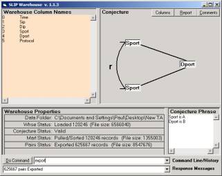
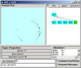
Figure 1: The Warehouse Browser after the SSI data
set is pulled and exported
This Exercise is followed by the introduction of the SLIP
Event Browser in the next Exercise.
Part
1: Use Warehouse to build the Analytic Conjecture.
This exercise requires a single zip file called ELE.zip. This file is 914K and can be
obtained from Dr. Prueitt at beadmaster@ontologystream.com.
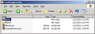
Figure 2: ELE.zip contains two zip files.
When the two zip files in ELE.zip are unzipped one will have a folder
that looks like Figure 2. The two
Browsers are in the folder “filtered”.
They can be copied and moved and require no installation.
Start with only the two browsers in an empty folder. Create a Data folder and place the
Datawh.txt, of your choice, in that folder. (Or just unzip the file filtered.zip). Launch the Warehouse Browser
(SLIPWhse.1.1.3.exe) and select any two of the column names (that make
sense). In our data set the Sip (Source
IP) is always spoofed and so the address is always 0.0.0.0. Moreover time has no repeated values so time
is not a particularly interesting column with respect to an analytic
conjecture.
The conjecture might be (b, a) = (Dport, Sport) as in
Figure 1. (Sport, Dport) might also be
interesting as would be (Dport, Dip), (Dip, Dport), (Dip, Sport) and (Sport,
Dip). (Spot, Protocol) produces too
many pairs to work with. However, a
secondary aggregation process will reduce the data representation. We use a category abstraction to produce
event templates (see Part 4), in this case a template selecting every 10th
record.
To make the conjecture (b, a) = (Dport, Sport) use the
commands
b = 4
a = 3
followed by the command
pull
export
“Pull” pulls the two columns into a file called
Mart.txt. “Export” computes and exports
the pairs of linked atoms from a temporary internal data structure to a file
called Paired.txt.
At present there are two Browsers. The SLIP Technology Browser was the first
developed. The Technology Browser
initially relied on FoxPro programs to produce four data files. In early December, we completed the SLIP
Warehouse Browser.
This Exercise reviews how a completed SLIP Framework is
produced. First take filtered.zip and unzip into an empty folder.
Now open the Data Folder and remove A1 (completely) and the files,
Conjecture.txt, Mart.txt, and Paired.txt.
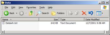
Figure 3: Datawh.txt alone in the Data Folder
Once you have used the Warehouse Browser to create the
files Mart.txt and Paired.txt, then launch the SLIP Technology Browser
(SLIP.2.2.2.exe). The imported files
are very large (6 Megs of data) so the application may take up to a minute to
open.
Once opened the user needs to type in the two commands:
Import
Extract
“Import” imports pairs from Paired.txt into an in-memory
database. “Extract” extracts atoms from
the Paired.txt by parsing the text and identifying unique values. For each value there will be one of more
occurrences of this value. An abstract
category is defined that binds all of these common values what is then called
an “atom”.
The number of records involved in this Exercise is
large. Under the Analytic Conjecture
(b, a) = (Dport, Sport), the initial 120,246
Audit records produce 626,668 pairs of atoms – each
pair having one or more link relationships via a “b” value. The extract command produces 1456
atoms. Note that 1456*1455 = 2,118,480
is the size of the set of all possible pairs.
(There are 1456 ways to fill the first part of the pair and then 1455
ways to fill the second part of the pair.)
Note also that the ratio 626,668/2,118,480 should be looked
at carefully. This seems to indicate
the normal operation of a LINUX kernel where there is no pre-selection of
events as being “intrusions” by an Intrusion Detection System such as RealSecure. However, there is a question about whether
or not there is some redundancy in the Paired.txt. From the theory of distributions, one knows that this number has
redundancy and needs to be removed by the Warehouse Browser before writing out
to the Paired file.
This can be done in a number of ways. Once this is done that the ratio will become
more meaningful as a measure of the anomaly in this data set.
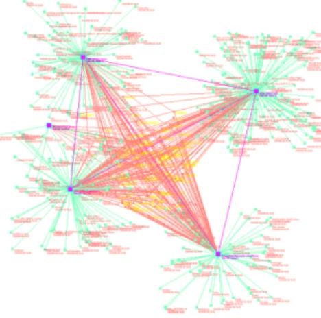
If your Analytic Conjecture is (Dport, Sport) then
clustering the atoms will produce a large cluster and a residue. Some
experimentation will show that this behavior is typical of this data set no
matter what the Analytic Conjecture and no matter what the scale of the data
set sampling template (see Part 4).
One of the reasons for a spike of this type may be simply
the size of the Audit Log. Having 120,000 records may simply connect link
relationships into a single event. But
the behavior appears also in random subsets of the data. So the single spike is likely the normal
signature of the system. One has to
look into the event.
A number of approaches are possible.
Part
2: Look into the Residue
First we may look outside the main event to see a number of
small events that are separated completely but that have very little (or
nothing to do structurally with the single main event.)
a b
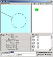
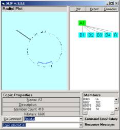
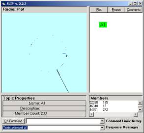
Figure 4: Clustering shows a main event having
1216 of the 1456 atoms and a residue
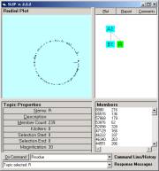
Clustering the residue will produce choices for 5 – 10
small groups of links atoms (primes).
The user can look for these him/herself. Type:
random
cluster 2000
This will randomize the distribution and then iterate the
gather process 20,000,000 times.
Once you have a small cluster identified and parceled into
a category, the Report will show the actual linked relationships.
To create a category, select a node, and show the
Plot. Use the command “x, y -> name”
to take the atoms in the interval (x, y) and put them into the category named
“name”. Select the node and type
“generate”. Then click the Report button.
Since the groups are small one can easily see structure in
the Report. However the link structure
can also be represented as an event graph.
Once in this form, then the links themselves have a time stamp and thus
the evolution of the event can be shown in an animation by changing the colors
of the links to trace the evolution of the event.
The event graphs will be an important
part of the SLIP Technologies. But we
need about six weeks to complete the Event Browser. For now we take two of the largest events outside of the single
main event show in Figure 4a, show the report and a hand drawn revision of the
event map. (The data folder for this is
called twosmallevents.zip).
A note should be made that version 2.2.2
requires that one use the key command to key to the atoms column, 3 in this
case. Type “key 3” before generating
reports.
The generation of Reports is now a brute
force in-memory process. For the large
SSI data set, this takes a few minutes even for a small report.
The principles of RIB algorithms are
well understood by OSI and the conversion is being done now. Several weeks of work is required to replace
the brute force method with the fast RIB algorithms. Once this is done, the reports will be generated almost
instantaneously.
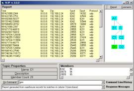
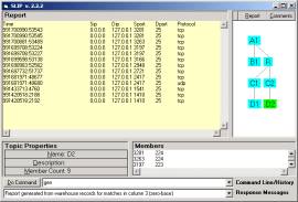
a
b
Figure 5: The Reports of two small clusters, in twosmallevents.zip
We look forward to seeing the features and properties that
OSI is putting into the SLIP Event Browser.
The Event Browser takes the next step.
The categories of a SLIP Framework can indicate the boundaries and exact
nature of an “event” that has occurred.
Event Chemistry is an active area of research at several
universities. The results of this
research are indicating that the event graph can be automatically generated
from a SLIP Framework category.
The Reports are viewed by the Browser but also can be
viewed by opening the Reports.txt file in the appropriate folder.
a b
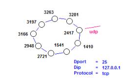
Figure 6: Two hand draw event maps
The hand draw event maps in Figure 6 are early
representatives of what the automated construction of event maps should look
like.
Note that Figure 6b looks like either a Port Scan or a
Trace Rout. However the nodes are
source ports not destination ports.
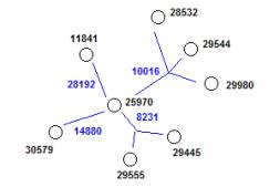
In Figure 6a the linked nodes <25970, 8231, 29555>
and <25970, 88231, 29445> both involve the destination port 8231. This means that the pairs of source ports
(925970, 29555) and (25970, 29445) are both linked by the destination port
8231.
Part
3: Look into the main event
The files needed by the SLIP Technology Browser are
pictured in Figure 5. The Warehouse
Browser requires only Datawh.txt. The
Warehouse Browser creates the files Conjecture.txt, Mart.txt and Paired.txt.
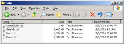
Figure 7: The files needed by the Technology
Browser
The use of the Technology Browser creates a folder A1 and
subfolders nested within A1. Child
nodes in the SLIP Framework have corresponding folders within the parent node.
From the single file, datawh.txt, one can create the SLIP
Framework developed in Figure 8. In
Figure 9 we show five primes, each of which should have an event map. The development of the event maps for this
data will be shown as soon as the Event Browser is completed.
The development of the Event Browser is important for a
number of reasons.
1)
The user
community will be able to parse Audit Logs into targeted event types that are
somewhat or completely isolated from the background noise.
a.
For
example, all port scans that are connected by a structural linkage will appear
as a linked circle such as in Figure 4b. Colored labels indicate the effected
systems.
b.
The
individual events will sometimes be linked weakly by links that are “external”
to the event, and thus identify sequences of events
2)
The
automated conversion of the event graph to a Petri net will allow the update of
event detection rules
3)
The
temporal coding of the links comes with the time stamp. With the use of timestamps we will be able
to see the order in which the nodes of the graph have been traversed.
4)
The
patterns expressed in the picture of the graph will become event clues that
will act as rapid informational retrieval.
“Find things that look like this” will produce information retrieval
during trending analysis and even in real time response analysis
The development of a set of graphical pictures of event
types will alter fundamentally the way in which incident response and trending
analysis occurs in the computer security organization such as the government
CERTs.
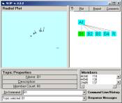
In Figure 8, interesting segments of the circle are
identified using the bracket indicator.
The command “x, y -> B1” creates the category B1, for example.
a
b c d
e f
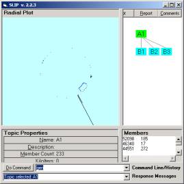
Figure 8: The A and B levels of the SLIP
Framework
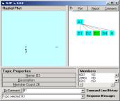
Each of the B level categories can be inspected for prime
structure. The derivation of these
prime structures is an art form. The
identification of a prime has a formal correspondence to the identification of
an actual event that is occurring in the natural world.
The ending nodes in Figure 9 are indeed prime. Look into each of these categories,
randomize and then cluster to check this.
If all atoms move quickly to the same location, then the category is
prime.
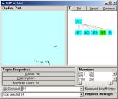
In the case of D1 and D2 these are derived from C3 and C5 by removing
atoms that are outside of the prime.
This is done by inspection and the use of the bracket command “x, y
->”.
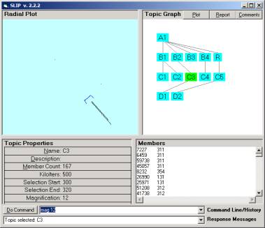
Figure 9: The complete SLIP Framework
The purpose of obtaining prime structures is related to the search for
means to separate data into events.
The events are then pictured as event graphs. Animation of the temporal sequence of the occurrences of links
produces a visual impression of how the event unfolds.
The user is encouraged to work with the data set in twosmallevents.zip or in the much smaller data set filtered.zip. twosmallevents.zip has the very large dataset discussed in Part 1 and
2. The two small events are those
represented in the event graph in Figure 6.
Part 4: Filtering the data to produce substructure
The data set filtered.zip
contains a datawh.txt that is filtered from the 120,246 records. Simply taking every 10th record produces
12,024 records. One should compare
Figure 8 with Figure 4.
a b
Figure 10: The filtered SSI
data
This data set is very easy to work with because the data size is
small. Moreover, the production of a
record set for import into the Warehouse demonstrates various techniques.
1)
Gain a representative
set of records, but of a size that makes visualization easy.
2)
Detect rare events
even in large data sets without visualization
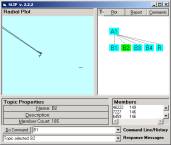
The dynamics of the cluster of A1 is important to note. First a spike develops. Then a group gathers together and moves
slowly towards the spike. As it moves
forward the group and the spike periodically exchange a number of atoms. The exchange process is captured in Figure 8
a and 8b.
The data set filtered.zip
contains the distributions show in Figure 10.
The three Reports have an event graph.
This event graph will be the first automatically generated event graph
and will be available in the next exercise.