SLIP
SLIP
Warehouse Exercise I
December 2, 2001
Obtaining Informational Transparency with Selective Attention
Dr. Paul S. Prueitt
President, OntologyStream Inc
December 2, 2001
SLIP Warehouse Exercise I
December 2, 2001
Index
Overview 3
Section 1: The use-case 4
Section 2: Exercise Part 1 6
Section 3: Exercise Part 2 11
Section 4: Exercise Part 3 18
Section 5: Exercise Part 4 20
Section 6: Return to use case analysis 25
SLIP Warehouse Exercise I
The following exercise uses the WinZip file swSLIP.zip. In the zip file there are two programs and a Data file. The program SLIP.2.2.2.exe is 344K and SLIPWhse.1.1.1.exe is 172 K. Neither requires an installation process.
The exercise is focused on the internal relationships between the records in an IDS Audit Log. A use-case analysis establishes an imagined context for the exercise (see Section 1).
The exercise has three parts:
Part 1 uses the Technology Browser to create three categories from the three major clusters of the top category node A1. A residue is computed and this residue is studied for event map candidates.
Part 2 removes the dataset used in Part 1. The Warehouse browser is then used to re-create the same dataset seen in Part 1. The data is again removed and a completely new Analytic Conjecture is developed and used to produce a different view of the IDS Audit Log. This view is about a subset of the Audit Log. In Part 2 we identify the critical notion of a kernel pattern.
Part 3 takes a new Analytic Conjecture and produces a Report using a different search column. The Report is a subset of the IDS Audit Log. This Report is then used by the Warehouse Browser to produce a refined view of the filtered Audit Log.
Part 4 re-examines the kernel patterns found in Part 2 and Part 3.
An event map of a single distributed event is drawn. The last section (Section 6) reviews the question of SLIP Technology relevance to items in the use-case analysis.
Section 1: The use-case
This
exercise will follow an imagined use-case scenario, as follows:
A phone call is made to a team officer regarding unusual activity that involves a number of Defense Department systems. The team Officer is asked to investigate.
U.1:
Following workflow, the team Officer begins a review Process.
U.1.1: Information about the effected systems is
reviewed.
U.1.2: Some initial requests for additional
information and verification of existing information are made.
U.1.3: The virus knowledge base is reviewed and it
is determined that neither a worm nor virus is primarily the cause of the
activity.
U.2:
Based on U.1.3 and the distributed nature of the activity, the team officer
conjectures that a coordinated cyber warfare attack is occurring.
U.3:
Requests for information regarding Security, Procedure, Legal and Policy issues
are made.
U.4:
An Incident Ticket is open and preliminary data and summaries are placed into the
Incident Ticket System.
U.4.1: At a different level of organization, Incident Ticket Management
(ITM) acknowledges that a new Ticket is open.
U.4.2: Trending analysis by ITM is performed once a day on
tickets that have been closed.
U.4.3: Open tickets are compared to trend profiles to
anticipate the next phase of the now conjectured cyber warfare event.
U.5:
A number of low impact sensor tools are deployed
U.5.1: A mobile DIDS (Distributed Intrusion Detection System) is
brought on line.
U.5.2: Mainline IDS systems are modified so as to selectively ignore the activity imposed by active self-scanning and intrusions.
U.5.3: The effected systems are scanned and a model
of open ports, and other easily accessible information is re-acquired to produce
a system state for state transaction analysis.
U.6:
Event boundaries are marked and a log file is made to record the activity of
the battery of low impact sensors.
U.7:
Audit logs from effected IDS systems are copied to an Audit Log Warehouse and
tagged with metadata.
U.7.1: Audit Logs are copied to match the best estimate of the
beginning and end of events. This best
estimate is to be refined so time stamps are maintained in an event table, with
keys into the primary copy of the Audit Logs.
U.7.2:
As better estimates of the beginning and end of events are developed, then
complete copies of the Audit Log from these periods of time is made and
isolated for study using SLIP.
U.8: At his point the response is split into two
groups:
U.8.1:
The real time response group actively works the Incident Ticket.
U.8.2:
The trend analysis group develops a global understanding of the event in the
context of all other Incidents, both open and closed.
U.9: The incident is
considered to be over and the analytic processes completed, so the Incident
Ticket is closed.
U.10: Incident Ticket
Management (ITM) acknowledges that an open Ticket has been closed.
Primary
use of SLIP can be made at: U.4.2, U.4.3, U.7.2, U.8.1, U.8.2.
The objective of this exercise is to familiarize the user with the tools that may be made available to Regional team, and to do so in a context that compares the SLIP Browsers with other tools generally available from data visualization, pattern matching, data aggregation, algorithmic categorization and machine learning technologies. A technical comparison is not made due to limited resources.
The development team is not fully aware of the internal details of team workflow, due to security issues. However, we can anticipate that the five use-case items listed in Table 1 is representative of the client’s critical and urgent need for new methods.
Table 1: Use-case items
U.4.2: Trending analysis by ITM is performed once a day on tickets that have been closed.
U.4.3: Open tickets are compared to trend profiles to anticipate the next phase of the now conjectured cyber warfare event.
U.7.2: As better estimates of the beginning and end of events are developed, then complete copies of the Audit Log from these periods of time is made and isolated for study using SLIP.
U.8.1: The real time response group actively works the Incident Ticket.
U.8.2: The trend analysis group develops a global understanding of the event in the context of all other Incidents, both open and closed.
After the three parts of this exercise are completed, then we will return to the question of how the SLIP technology might be used, if widely deployed.
Section
2: Exercise Part 1
Part 1 uses the Technology Browser to create three categories from the three major clusters in the limiting distribution for the top node A1. A residue is computed and this residue is studied for event map candidates.
If you have the zip file swSLIP.zip then you may uncompress the files into any empty folder on your computer.
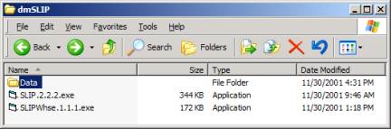
Figure 1: The un-zipped files from swSLIP.zip
The Data folder need only contain one ASCII file called datawh.txt. However, the files and nested folders that you have unzipped have been developed to show specific data invariance.
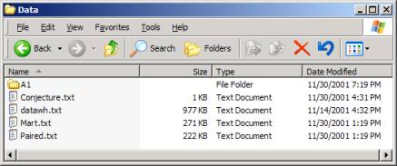
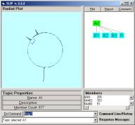
Figure 2: The Data folder’s contents
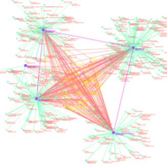
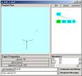
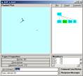
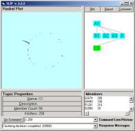
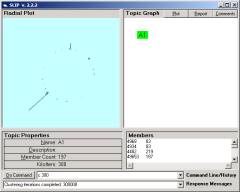
Check to see that your folders have the same contents as in Figure 1 and 2. Navigate back up to the SLIP.2.2.2.exe and double click on the icon. The browser will traverse all nested folders in the Data folder and produce a visualization of the cluster pattern seen in Figure 3a. Category A1 contains 877 atoms. These are defined as those d_port values in an Analytic Conjecture that links into pairs due to there being a common source IP address shared between the two d-port values. To understand the Analytic Conjecture better, one can review the SLIP Technology Browser Exercises, or look at the next section of this Exercise. These exercise sets are available on CD-ROM from OntologyStream Inc.
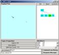
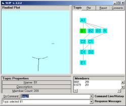
In Figure 3 the Browser displays nodes at the A and B levels. A1 is the original set of 877 atoms developed from a complete analysis of the 14,276 records we have in the IDS Audit Log. B1, B2, and B3 are taken from the three large clusters seen in Figure 3a. R is the residue category that contains the complement of the union of the other three categories in level B.
a

b c d e
Figure 3: The A and B levels of a SLIP Framework
The user can use the SLIP Browsers to develop a similar Framework. The Technology Browser Exercises shows more about how this is done. However the development of categories will be reviewed in part 2 of this Exercise. Part 2 will also show how to set up the data files needed by the Technology Browser. The Warehouse Browser is used to create these files.
What we are interested in Part 1 of this Exercise is the category R. In previous exercises and experiments we have noticed that small structure can be found outside of the larger structures by clustering the group A1 sufficient to produce major clusters, and then removing these clusters from consideration. The residue function does this by selecting the A1 node and typing “residue” in the command line. The user will be asked to complete a similar exercise in Part 2.
When the residue is first placed into the category R the atoms are kept at the location as they where in the A1 distribution. One can randomize the atoms or simply let them be where they are. We are looking for a limiting distribution having a fixed-point property. By typing 4300 (4,300,000 iterations) we see that the atoms move around and then begin to settle into one location. This number of iterations would take several hours in the original prototypes developed in FoxPro. However, by using our In-Memory search algorithm, the iterations take around a minute before all motion stops.
A dedicated In-Memory database and data base management system has been created to enable the SLIP Technologies.
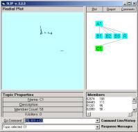
In Figure 3e we use the line command “70,111 à C1” to put 58 atoms into a single category. In Figure 4a we see the detail of the structure. This structure is not changing with additional iterations so we can feel comfortable that this structure is an invariant under additional iterations. We also see that there are two gaps that produce what appear to be three separated groups. We want to build event maps for these three groups and determine but internal group linkage and inter group linkage (if any).
a b
Figure 4: Category C1
In your data set you will not see Figure 4a since we have clustered this group to produce the distribution in Figure 4b. What we learn is that in this limiting distribution any separation (of more than one degree) really represents a cluster where there is no external linkage to any other cluster. This is due to the fact that the distribution is stable, so that further iterations will not move any atom’s location. Theorems regarding stable distributions are found in my published work.
The user can recreate the large spike in Figure 4a. One may randomize the atoms distribution and re-cluster the category C1. All of the other atom groups will be show to be not related in any way (in Category C1) to those in the spike. This fact can be checked by hand, or be repeatedly randomizing and reclustering. The pattern is invariant.
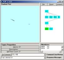
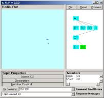
As an exercise one should select one of the larger clusters and create categories and various reports for those categories. We selected the largest categories at [153, 158] and [340, 345] and put them in categories D1 and D2 with the commands “153, 159 à D1” and ‘340, 345 à D2”.
a b
Figure 5: Categories D1 and D2
In category D1 there are 27 atoms. In category D2 there are 4 atoms. Category D1 is not prime, sense that there are two groups of atoms that are not linked. One can see this by generating a Report from the original IDS data.
The reports for any category can be generated by selecting the category node and typing “generate” in the command line. If one selects the Report function first one can see the delivery of IDS Records into the Report as the sort and search algorithms run.
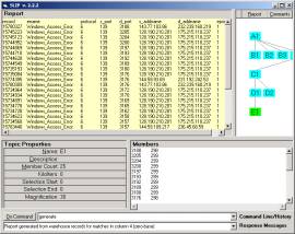
Figure 6: The Report for Category E1
The IDS records :
record ename protocol s_port d_port s_addname d_addname epriority
15779608 DNS_Length_Overflow 17 53 34608 141.190.129.252 164.59.101.3 1
15779609 DNS_Length_Overflow 17 53 34608 141.190.129.252 164.59.101.3 1
15773215 DNS_Length_Overflow 17 53 32834 198.49.185.110 163.77.12.19 1
15773170 DNS_Length_Overflow 17 53 32834 198.49.185.110 163.77.12.19 1
15773191 DNS_Length_Overflow 17 53 32834 198.49.185.110 163.77.12.19 1
15773200 DNS_Length_Overflow 17 53 32834 198.49.185.110 163.77.12.19 1
15773201 DNS_Length_Overflow 17 53 32834 198.49.185.110 163.77.12.19 1
15773214 DNS_Length_Overflow 17 53 32834 198.49.185.110 163.77.12.19 1
15779612 DNS_Length_Overflow 17 53 32834 141.190.129.252 163.77.12.18 1
15779613 DNS_Length_Overflow 17 53 32834 141.190.129.252 163.77.12.18 1
The d_ports 34608, 32834, having the s_port 53 in common. All other 25 atoms in category D1 have the s_port 139 in common. However, s_port is NOT involved in the Analytic Conjecture, source IP address is. The data here indicates the potential value to a new analysis model that is suggested in Part 3 of this Exercise.
Ok, so now what?
First, it can be pointed out that the Report is a subset of the Audit Log records. These records contain information regarding IP addresses, protocols, and the record number. Any drill down capability available through the Audit Log is available to the user.
Second, it is true that one can take a composite of Reports and use the Warehouse Browser to create a different view of the data using a different Analytic Conjecture. All relationships and facts found in this way are real facts and real relationships that exist and characterize this specific data set.
Third, we will soon have both event map representation and the representation of atom valance to work with in producing a highly recognizable visual form to event and sub-events within this dataset.
Event map formation will soon be fully automatic so that Audit Logs can be represented using atomic and compositional event maps. Manual control of event map construction will also allow the user to modify relationships to reflect
1) Missing data
2) Conjectures and
3) Tacit Knowledge
Visual inspection will locate similarities between incidents. Once similarity is recognized then a data drill down is easy.
We these comments will have to be addressed more fully in later Exercises.
Section 3: Exercise Part 2
Part 2 of this Exercise removes the Part 1 data set completely. The Warehouse browser is then used to re-create the same data set seen in Part 1. The data is again removed and a completely new Analytic Conjecture is developed and used to produce a different view of the IDS Audit Log.
Before deleting the data in the Data folder we should concatenate an interesting Report. Let us take the Report from category E2. Move this file to the folder show in Figure 1. Now use the Technology Browser and select one of the three large categories, say B1. The category B1 has 209 atoms. Look at Figure 3b and notice that surrounding atoms are included even though they are outside of the single strong spike.
Now generate the Report for Category B1 using the “generate” command. The browser has excellent event loops so one can click on the Report button to see the generation of the individual Audit log records even during the execution of the generate command. The generate command takes the first atom, 8001, and generates all matches to atom from the Audit Log. Then the generate command takes the next atoms and so further. An “order atoms” command, not implemented as yet, nicely orders Report columns as we need.
Combine the two Reports to use in Part 4 of this Exercise. You will need to cut and paste one of the files and add this to the other file and then rename the joined file using the name “datawh.txt”. Put this aside.
It should be noted that the generate command uses refined search and sort algorithms that produces fast results and does not depend on a third party database management system. These algorithms are available in the code, but have not been fully documented as yet.
Now delete the folder A1 and all of its contents. Delete the files Conjecture.txt, Mart.txt and Paired.txt. Only Datawh.txt should remain in the Data folder. Datawh.txt contains the original 14,473 IDS Audit Log records.
a b
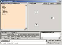
Figure 7: Opening the Warehouse Browser with the help file (not in scale)
We now demonstrate that we need only a tab-delimited file that contains any Audit Log, or any event log. Double click on SLIPWse.1.1.1.exe (in Figure 1). You should have only the 977K file, Datawh.txt, in the Data Folder.
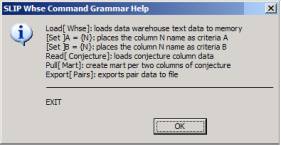
After opening, Warehouse Browser will look like Figure 7a. By typing “help” in the command line you find the set of commands (Figure 7b). We need only use the following commands:
· Set b = 3
· Set a = 4
· Pull
· Export
You will see a response in the Response Message lines:
· Mart data Pulled, containing 14473 records.
· 137493 pairs Exported
as well as other messages displayed and stacked in the Response Message line. Click on the small control to the right of the Command line and the Response Message line.
You now have a Paired.txt to use with the Technology Browser. You can now close the Warehouse Browser. Additional functions will be explored later.
Look into the Data Folder and you will see new Conjecture.txt, Mart.txt and Paired.txt files. Now double click on the SLIP.2.2.2.exe icon to see Figure 8a.
a b
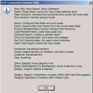
Figure 8: The Technology Browser and its Help file
The Import and Extract commands should be issued to develop the atoms of the top node and to randomly distribute these to a circle. One can see the result by clicking on the A1 node.
We want to cluster until we reach a limiting distribution where nothing is moving. Try 30,000,000 iterations, so type “cluster 30000” (K = 1,000). This will take around 20 mins. While you are waiting you might enjoy changing the magnification by typing in “mag 10”, “mag 2”, or ”mag 200”. Internal event loops handle this just fine. Of course, most of the cluster structure is seen in a few seconds.
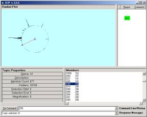
Figure 10: The limiting distribution of Category A1
The limiting distribution finally stops movement, after a long period of fine structure changes. More will is on the stochastic and categorical formalism in private research notes.
One can use the zip file to put a copy of the Part 1 exercise data into an empty folder and look again at category E1 (Figure 6). We can see that the 25 atoms of E1 contain the atom 3188. In Figure 10 we may use the indicator line to point to this atom and notice the small cluster containing 3188. (Your picture will have this cluster at a different location.)
Make a category from the single cluster containing 3188. Scroll down the members list to find the atoms 3188 and its location. Then use the indicator line by typing just the location into the command line. Use the bracket function to get the single spike and any other spikes that are very close by. After putting these into a category B1 then randomize and cluster this collection.
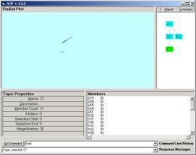
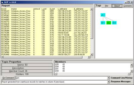
Figure 11: The Prime C1 containing 31 atoms
The category E1 (Figure 6) has 25 atoms each sharing source port 139. The interesting correlation is that the Analytic Conjecture that we used to create this data set uses the source IP address as the non-specific relationship and the d_port as the atoms.
Table 2
record ename protocol s_port d_port s_addname d_addname epriority
15745434 Windows_Access_Error 6 139 3210 128.190.210.201 175.215.110.237 1
15745323 Windows_Access_Error 6 139 3208 128.190.210.201 175.215.110.237 1
15745223 Windows_Access_Error 6 139 3205 128.190.210.201 175.215.110.237 1
15745123 Windows_Access_Error 6 139 3204 128.190.210.201 175.215.110.237 1
15745042 Windows_Access_Error 6 139 3201 128.190.210.201 175.215.110.237 1
15744952 Windows_Access_Error 6 139 3200 128.190.210.201 175.215.110.237 1
15744869 Windows_Access_Error 6 139 3197 128.190.210.201 175.215.110.237 1
15744771 Windows_Access_Error 6 139 3196 128.190.210.201 175.215.110.237 1
15744710 Windows_Access_Error 6 139 3193 128.190.210.201 175.215.110.237 1
15744628 Windows_Access_Error 6 139 3192 128.190.210.201 175.215.110.237 1
15744549 Windows_Access_Error 6 139 3189 128.190.210.201 175.215.110.237 1
15735193 Windows_Access_Error 6 139 3180 128.190.210.201 175.215.110.237 1
15735084 Windows_Access_Error 6 139 3176 128.190.210.201 175.215.110.237 1
15774395 Windows_Access_Error 6 139 3176 144.59.93.69 231.192.242.53 1
15780309 Windows_Access_Error 6 139 3176 143.77.103.86 232.239.160.219 1
15735019 Windows_Access_Error 6 139 3173 128.190.210.201 175.215.110.237 1
15734964 Windows_Access_Error 6 139 3172 128.190.210.201 175.215.110.237 1
15734934 Windows_Access_Error 6 139 3170 128.190.210.201 175.215.110.237 1
15734891 Windows_Access_Error 6 139 3169 128.190.210.201 175.215.110.237 1
15734778 Windows_Access_Error 6 139 3165 128.190.210.201 175.215.110.237 1
15734728 Windows_Access_Error 6 139 3162 128.190.210.201 175.215.110.237 1
15734670 Windows_Access_Error 6 139 3161 128.190.210.201 175.215.110.237 1
15734623 Windows_Access_Error 6 139 3158 128.190.210.201 175.215.110.237 1
15734568 Windows_Access_Error 6 139 3157 128.190.210.201 175.215.110.237 1
15783440 Windows_Access_Error 6 139 3157 144.59.109.217 236.45.68.59 1
15783443 Windows_Access_Error 6 139 3157 144.59.109.217 236.45.68.59 1
15734516 Windows_Access_Error 6 139 3153 128.190.210.201 175.215.110.237 1
15734427 Windows_Access_Error 6 139 3152 128.190.210.201 175.215.110.237 1
15734358 Windows_Access_Error 6 139 3149 128.190.210.201 175.215.110.237 1
15734273 Windows_Access_Error 6 139 3148 128.190.210.201 175.215.110.237 1
15734193 Windows_Access_Error 6 139 3145 128.190.210.201 175.215.110.237 1
15734097 Windows_Access_Error 6 139 3144 128.190.210.201 175.215.110.237 1
15734066 Windows_Access_Error 6 139 3141 128.190.210.201 175.215.110.237 1
15734015 Windows_Access_Error 6 139 3140 128.190.210.201 175.215.110.237 1
15733980 Windows_Access_Error 6 139 3137 128.190.210.201 175.215.110.237 1
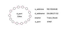
3210, 3208, 3201, 3173, 3161, 3140 are the six atoms that are in Figure 11 but not in Figure 7. So how can we determine exactly why these are not in Figure 7? First let us denote the cluster in Figure 11 as category C*. Then we hand draw the event map in Figure 12. This event map is derived soley from the Audit Log records seen in Table 2.
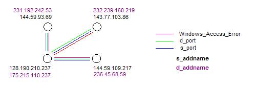
Figure 12: A kernel event map for category C*
So far the developers of SLIP have found several event maps that have complex properties.
By complex we mean that single formal structures have a small number of multiple but specific interpretations. What might be implied by these findings is that there is a program that is run in different contexts or at different times. The structure of these event map “kernels” would seem to indicate the actual structure of the program event cycles.
This implication is a strong implication but is consistent with both theoretical finding and with experimental evident that the development team has found so far. Finding (and writing about) these event map kernels takes a number of hours and has been mentally exhausting. However, the internal program event-loops and object definition already built into the Browsers will soon allow automated production of event maps of the type seen in Figure 12.
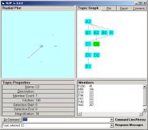
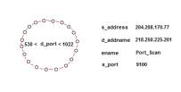
Figure 13: A cluster of 7 elements containing 3110, 3161, 3140
In Figure 13 we find part of the missing six atoms as well as a small cluster that is isolated (see discussion under Figure 10). This cluster of 7 atoms is in fact not prime, but clearly there is a structural relationship to C*. Generating the report on Figure 12 helped us begin the process of specifying this structural relationship.
Table 3
record ename protocol s_port d_port s_addname d_addname epriority
15732480 Trace_Route 6 80 51200 202.96.106.11 167.198.122.103 2
15773893 Trace_Route 17 16590 51200 4.2.55.114 163.77.20.105 2
15735637 Windows_Access_Error 6 139 4355 155.215.187.109 149.29.47.186 1
15745434 Windows_Access_Error 6 139 3210 128.190.210.201 175.215.110.237 1
15744771 Windows_Access_Error 6 139 3196 128.190.210.201 175.215.110.237 1
15734670 Windows_Access_Error 6 139 3161 128.190.210.201 175.215.110.237 1
15734015 Windows_Access_Error 6 139 3140 128.190.210.201 175.215.110.237 1
15729990 TCP_Overlap_Data 6 80 1692 207.246.136.108 151.92.226.140 1
15759612 Stream_DoS 6 80 1692 209.132.14.123 175.215.33.137 1
This report presents a number of issues, which are taken up in Part 3 and Part 4 of this exercise.
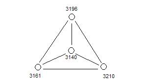
The subset 3210, 3196, 3161, 3140 is prime.
Table 4
15745434 Windows_Access_Error 6 139 3210 128.190.210.201 175.215.110.237 1
15744771 Windows_Access_Error 6 139 3196 128.190.210.201 175.215.110.237 1
15734670 Windows_Access_Error 6 139 3161 128.190.210.201 175.215.110.237 1
15734015 Windows_Access_Error 6 139 3140 128.190.210.201 175.215.110.237 1
A few observations:
- The d_port 3210, 3196, 3161 and 3140 each have only one IDS Audit record.
- These four d_ports are involved in a highly unusual pattern as depicted in Figure 13 and 14.
- The structural linkage that involves these four ports can be computationally identified (See Part 4 of this Exercise).
-
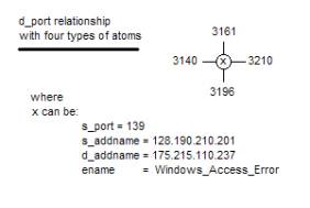
Figure 13: a kernel condition depicting a pattern of interest
These four d_port values might be regarded as a kernel, where the notion of a kernel is some minimal structure that is used to generate something more fully.
![]()
![]()
![]() Figure 14: The event map a kernel
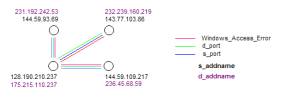
Figure 14: The event map a kernel
Figure 14 shows a graph of the same information represented in Figure 13. What is surprising here is that this single graph can be labeled with three types of links: the s_port 139, the s_addname 128.190.210.201 and the d_addname 175.214.110.237.
A conclusion from this exercise is that we have found a kernel
event. The kernel event must involve an attack from 128.190.210.201
through port 139 against 175.214.110.237 using ports 3196, 3161, 3210 and
3140. But, of course, the attack is a
bit more complicated than this. The
linkage between Table 4 and Table 2 is only very small. 3210 is the first d_port in Table 4 and
3140 is the second to the last d_port in Table 4, but each atom 3210, 3140,
3161 and 3196 occur only once. The
event map kernel in Figure 12 involves four sets of d_addnames and s_addnames,
where as the event kernal in Figure 14 involves only the single d_addname
128.190.210.201 and the single
s_addname 175.215.110.237
.
Our conclusion is that these two kernels are the structure of two different phases of the overall attack. We will return to this issue in Part 4 of this Exercise.
Section 4: Exercise Part 3
Part 3 takes a new Analytic Conjecture and produces a Report using a different search column. The Report is a subset of the IDS Audit Log from April 15th, 2001. This Report is then used by the Warehouse Browser to produce a refined view of the filtered Audit Log.
We start by taking the Report on Category B1 from Part 2 of this Exercise. We create an empty folder and copy the two SLIP Browsers into that folder. Then create the Data folder put the file into this folder. Rename this file as datawh.txt. The Report from category B1 is now substituted for the full 14,337 IDS records.
a b
Figure 15: The re-use of a Report as the Warehouse
· Set a = 5
· Set b = 1
· Pull [create Mart.txt based on (b, a) ]
· Extract [use a combinatory algorithm to create Paired.txt]
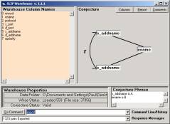
Figure 16: The use of the Warehouse Browser to create Analytic Conjectures
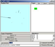
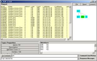
Figure 17: Drill down into a prime structure
One can look to see if each of these two clusters really represents “separate” events.
This is left as an exercise.
Section 5: Exercise Part 4
Part 4 of this Exercise set more fully develops the notion of event maps, kernel events and event chemistry. The completed data set is in P4_SLIP.zip.
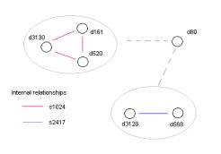
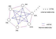
Figure 18: Some early event maps
Check B1 union E1
The reports for category B1 and E1 (Figure 5 and 6) where removed before making the zip file, swSLIP.zip, so the user will have to create these two file before starting this Part of the Exercise.
After generating both files, combine them by adding the records of one of the files to the records of the other file. Be sure not to add the header twice or to introduce a blank line.
Move the new file somewhere safe (see Figure 19). Now delete the folder A1 and all of its contents. Delete the files Conjecture.txt, Mart.txt and Paired.txt. There should be nothing in the Data folder at all.
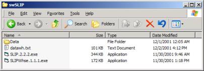
Figure 19: swSLIP folder with a new datawh.txt
The new datawh.txt should be of size 101KB. Move this file into the Data folder and start SLIP Whse.1.1.1.exe.
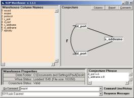
Figure 20: The Warehouse Browser
Use the commands:
- B = 5
- A = 4
- Pull
- Export
These commands instruct the Warehouse Browser to develop Paired.txt. Paried.txt is developed using the SLIP In-Memory database management system and a combinatorial algorithm. Paired.txt is the set of all d_ports that have a common s_addname value and thus has a so-called non-specific linkage.
This is a shallow link analysis. Shallow link analysis is very useful, but the Warehouse Browser can support that more complicated link analysis. This will be explored next year.
Now look into the Data folder to verify the change made. Then move back to the SLIP.2.2.2.exe and open the Technology Browser. Use the commands:
- Load
- Extract
The Load command instructs the Technology Browser to Load the Paired.txt and Datawh.txt into the SLIP In-Memory database. The Extract command instructs the Technology Browser to extract the uniquely defined set of atoms from the Paired.txt.
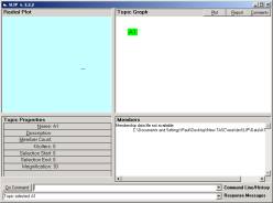
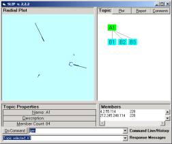
Click on the node A1. One will see Figure 21a. Cluster these atoms to find the characteristics of the limiting distribution. Your distribution will be similar to Figure 21b.
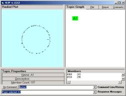
a b
Figure 21: A1 clustering
The three main clusters are parceled off into categories B1, B2, and B3 and a residue computed. Then each of the non-residue categories are randomized and re-clustered to eliminate all but the prime part of the cluster. B3 had two primes and so these are separated into C3 and C4.
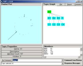
Figure 22: The SLIP Framework find in Part 4 Data.zip
Combine the reports for category B2 and E1 (Figure 5 and 6). swSLIP.zip, has this data.
Create an empty folder, put the two browsers in that fold and create a Data fold and put the combined file into that Data folder. Rename the file to “datawh.txt”.
Use the Warehouse Browser commands:
- B = 5
- A = 4
- Pull
- Export
to develop Paired.txt.
Use the Technology Browser commands:
- Load
- Extract
The SLIP technology will become valuable to the team
community IF it is field tested and then deployed as part of an effort to
integrate activity and analysis using a stratified taxonomy and information
sharing architecture. SLIP can
also be used as a personal research assistant without any integration.
SLIP was developed because the Consultant saw how a bridge might be made between the event records in IDS Audit logs and events as perceived by team analyst. These events are the substance of Incident Reports. The technical capability of the SLIP technology can be demonstrated within a project plan that might be developed for the first two quarters of next year.
Everything is on the table. However the finishing touches of the SLIP technology prototype need to be completed AND a limited field-test of the stand-alone executable needs to be made. This work can be completed during the month of December 2001. The field-testing would test the SLIP Browsers as a personal research assistant.
SLIP is not the final solution to all problems everywhere. But SLIP is new and powerful and it binds together the millions of IDS records generated each day into artificial constructs. These constructs include graphs that represent the real invariance in these data sets.
Use-case items
U.4.2: Trending analysis by ITM is performed once a day on tickets that have been closed.
U.4.3: Open tickets are compared to trend profiles to anticipate the next phase of the now conjectured cyber warfare event.
U.7.2: As better estimates of the beginning and end of events are developed, then complete copies of the Audit Log from these periods of time is made and isolated for study using SLIP.
U.8.1: The real time response group actively works the Incident Ticket.
U.8.2: The trend analysis group develops a global understanding of the event in the context of all other Incidents, both open and closed.
U.4.2: Trending analysis by ITM is performed once a day on tickets that have been closed.
Prueitt’s work on event trending goes back to the development of a trouble ticket analytic system for network performance in 1995. The client was MCI. The core problems with implementation and technology development are addressed in the Consultants current work. Event trending requires that a sign system or some taxonomy of concepts be acquired and shared within the Incident Management Team.
The event maps have a specific drill down capability into the Audit Log from which the event map is produced, as well as a specific drill down into any other Audit Log where a similar type event has occurred.
U.4.3: Open tickets are compared to trend profiles to anticipate the next phase of the now conjectured cyber warfare event.
When a ticket is opened team will identify one or more relevant Audit Logs. These Logs can be automatically processed to produce a pictorial representation of the link patterns within the data. Mechanical match will not often be possible. However human visual acuity will see similarities. The SLIP technology is easy to use and is un-encumbered with third party software. This allows the team specialist a freedom to explore rapidly potential commonalities between past events and the current event.
U.7.2: As better estimates of the beginning and end of events are developed, then complete copies of the Audit Log from these periods of time is made and isolated for study using SLIP.
The beginning and end of an event can be discovered using algorithmic means. These means are not so easy to simply talk about. They have to be developed by advanced computer scientists. The SLIP Browsers are designed to allow this type of experimental work on general methodology for event chemistry. The OSI sponsor can be in the position of having sponsored the development and deployment of these advanced means.
When the beginning and end of an event is know and the minimal parameters of the events are briefly described, the SLIP Browsers can fill out the details regarding the event. As team specialists read the training materials, they will identify new ways to represent distributed incidents as event maps.
U.8.1: The real time response group actively works the Incident Ticket.
SLIP does two things in real time. First, the visualization of large or small data sets is made easy since the graph structures of the events under study are pictures of real relationships in the data. No looking at long columns of data or data visualization where there is not underlying theory as to what event boundaries might look like. Second, the information that the response group is working with can be quickly manipulated with the SLIP Browsers to find some kernel pattern that can be discussed within the group. The community can work knowledge claims and knowledge validations with pictorial images as conceptual anchors.
U.8.2: The trend analysis group develops a global understanding of the event in the context of all other Incidents, both open and closed.
Again, SLIP is not the final solution to all problems everywhere. But it is new and powerful and it binds together the millions of IDS records generated each day into artificial constructs that represent the real invariance in these data sets.