Data
Structures, Theorems, and Programs
Obtaining
Informational Transparency with Selective Attention
Dr. Paul S. Prueitt
President, OntologyStream Inc
October 24-25, 2001
Shallow Link analysis, Iterated scatter-gather and Parcelation (SLIP)
Data Structures, Theorems, and Programs
Public Domain Materials
October 24-25, 2001
Introduction
Only tables and algorithms where involved in
the original SLIP experiments. There where
no relationships between tables.
Therefore the tables can be written as simple arrays. These can be stored in text files and mapped
into memory.
Due to our design principles, we are able to
move the entire SLIP technology into flat files and any programming language
like Java, C or Basic.
Data mining type operations can then be made
fast enough to allow creative interaction between a domain expert and a SLIP
Framework. For example, a SLIP
Framework now takes about four hours to develop, mostly because of manual
steps. The total run time is about 40
mins – mostly to do the gather process.
This run time can be reduced to 1 – 2 mins, perhaps less.
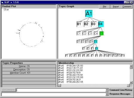
Figure 1: SLIP Interface 1.5, showing the radial plot
for category C5
The Framework is the stratified concept map
created through the human / SLIP interaction.
In developing the data transformation algorithms and other data
processing requirements, we separated the programs and data structures into
four groups.
In Section 1 we provide a software
specification for each of the four groups of programs and data structures. In Section 2, we begin the exposition of a
formal theory of categorization using the SLIP technology.
In Sections 3 and 4, we describe the existing
programs for doing the scatter gather and the parcelation of a set into
categories. The categories have been
shown to be event types. These event
types form a type of generalization and abstraction for single IDS events into
distributed, over time and location, IDS events.
Section 1: The Full Function SLIP, Software Specification
The full function SLIP interface needs all
four of these groups of algorithms and data structures.
Group 1: Set-up, Programs and Data Structures
1.1: Manually
create the SLIP Data Mart and the Analytic Conjecture
1.2: Produce an
interface between Visual Insights and/or data sources such as RealSecure (under
consideration)
1.3: The only
output is a single file with two columns and a written description of the
Analytic Conjecture
Group 2: Production of the Top level of the SLIP Framework, Programs and Data Structures (see Section 1)
2.1: Requires only
the two column SLIP datamart
2.2: Produces two
tables:
2.2.1: A table of Atoms involved in the non-specific relationship defined by the SLIP Analytic Conjecture
2.2.2: A table
called <Pairs> which is the set of atoms that are paired by the
non-specific relationship in the Conjecture
2.2: Automatically
clusters the set of atoms but does not produce a category membership (done)
Group 3: Parcelation, filling out the SLIP framework, Programs and Data
Structures (see Section 2)
3.1: Only requires
the set of atoms, A, and the set of pairs, P.
3.2: Iteration
automatically produces new levels in the SLIP Framework Tree (done)
3.3: Iteration can be manually applied under specific conditions to create modifications to the SLIP Framework (done)
Group 4: Enterprise management, Programs and Data Structures
4.1: Allows the
navigation and review of various existing SLIP Frameworks (Version 1.5
available as of Oct 16th, 2001)
4.2: Allows the
encoding of interpretation and comments about the SLIP categories (version 1.6
available Oct. 17th, 2001
4.3: Allows
additional parcelation due to manual use of Group 3 processes (under
development)
4.4: Has a small technology
footprint. No installation process and
no database. (under development)
4.5: XML encoding
and mobile agents allow very easy sharing of SLIP structures (under
development)
Section 2: Definitions and Theorems on the
decomposition of a SLIP data set
This is edited and extended from Section 6.8: “Definitions and Theorems on the decomposition of a SLIP data set” from the October Report: “Summary of Results: July – October 2001, SLIP Intrusion Detection Technology (74 pages).
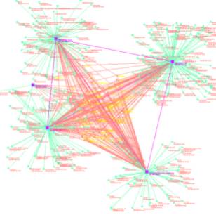
The SLIP technology does a Fourier type decomposition of all invariance in the data set into clusters that have tight inter-cluster linkage and weak intra-cluster linkage. This invariance is encoded as the nodes of a tree (see Figure 2).
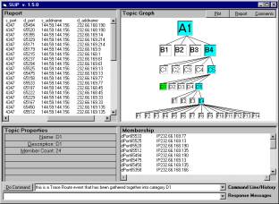
Figure 2: A trace route event that is gathered into category D1
In figure two we see the SLIP interface version 1.6 (October 17th, 2001). By scrolling the top left window we would see that a RealSecure IDS classified each of the 24 elements of category D1 as a Trace Route event. The only computational means for gathering these elements together is the non-specific relationship between Source IP plus Source Port and Target IP plus Target Port.
Observation 1: On the question of non-crisp categories:
The clusters themselves are gathered from the four limiting distributions. The set of all of these will have pairs of clusters that have non-empty intersections. What lies outside of a core might be considered to be an environment and may have significance. However, we focus first on the cores of these categories.
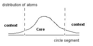
Figure 3: Characterization of a core
Our method for automatically generating a framework to start analysis was chosen to eliminate the environment. We are looking for what stays the same as one moves from one event type to another. The core is the center of a category where this center is invariant across several limiting distributions. The purpose of the SLIP Framework is to make available to domain experts the invariance that is produced by the non-specific relationship.
The set of ending nodes (sometimes called the leafs) of the SLIP Tree produces a crisp partition of the original set of atoms. This is because children are always produced in such a way as to provide this crisp partition with no overlap between the memberships of the children. The memberships of the children also will union to produce the complete membership of the parent node in the SLIP Framework tree. This is the important notion of disjoint union.
A series of theorems can be given. However, the observation now is that a non-crisp partition can be developed in order to reflect what we conjecture would be category entanglement (again look at the separation of context and core seen in figure 2).
In more advanced implementation of the fundamental SLIP theory, one can use feature analysis and a voting procedure to rout new events into a type of non-crisp classification based on profiles of categories. This introduces the notion of a tri-level architecture for information routing, categorization and information retrieval. These more advanced implementations await the completion of the first fully stand alone full function SLIP interface. The reason why we mention the advanced implementation is that when the SLIP Frameworks are being created and shared, then a number of intelligent programs will be possible.
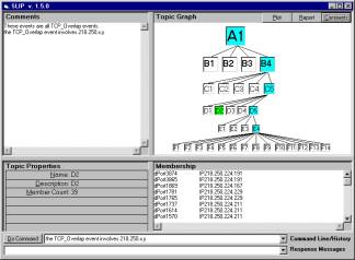
Figure 5: The SLIP Interface taking comments on an event category
The SLIP methods produce context free core category memberships that appear in different environments. The method is a direct intersection of sets rather than a statistical method.
Metadata can be associated with these nodes. This is done using a scripting language from the command line (see Figure 5). Comments made by analysts are appended to a file pointed by a metadata tag within the node tag in XML.
Observation 2: On the fundamental SLIP theory:
A set of definitions establishes an abstract mathematical language. This language is useful for two basic reasons:
1) The language allows one to conjecture about and prove properties that one can find experimentally by developing algorithms and software
2) The language allows a peer review of the underlying intuitions about what the SLIP technology might be used for (both in ID work and elsewhere)
Primary concepts:
Datamart: The SLIP datamart consist of a table with two columns. In the non-database version of the SLIP technology, an ACSII text file replaces the table.
The selection of the datamart is important. The following issues might have an impact on what type of data is selected and which records from a larger database will be used.
1) A time period may delimit an event or group of events.
2) A domain expert may analyze the nature of the data itself and produce an Analytic Conjecture. For example the first column value might be the defensive addresses and the second column value might be the system calls that occurred during the time interval in question.
It is important to realize that much of the value of the SLIP technology will come about when domain experts develop data with specific investigations in mind.
Non-specific relations
Pairs of first column values are identified by parsing the Datamart
and finding occurrences where a second column value (b) appears in more than
one record.
The critical issues are only that each line
in the Pairs text file represents a record and that the record represents a
single event.
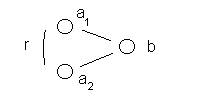
Figure 5: The
non-specific relationship between the atom a1 and a2
Two values from the first column are paired
if the associated value in the second column is the same. This situation is represented in Figure
5.
Once this pairing is done, then the pairs are
used to specify atoms. The atoms are
those elements that are in one or more pairs.
Formally we have:
( a1
, b ) + ( a2 , b ) à
< a1 , r, a2
>
where r is the non-specific relationship.
Pairs.dbf Pairs.dbf (formerly called Two.dbf) is the data source that contains the pairs of secondnames The table is denoted with a script bold Q.
Set of Atoms Q is parsed to
find all occurrences of second column values.
These are added into the Atoms.dbf.
This set is determined by the occurrences of the non-specific
relationship, and often times the set of atoms is a small percentage of all
second column values that are in the mart.
The percentage is sometimes 1/1000, for example. Thus a much larger data set is reduced in
size at the very beginning of the SLIP computations. The set of atoms is denoted with a script bold A. This reduction of data into “informational units”
is not statistical. Data aggregation is
a filtering process that uses the non-specific relationship to pull things that
are related but only related by this one well-defined non-specific
relationship.
All of this computational process is
formal. Not meaning is assigned until
the domain expert looks that the membership, using the membership to produce a
report from the original data source, and making human judgments about the
nature of the core category. These
judgments are then collected if the domain expert types into the comment
property of the core category.
The notions of nearness and the topological notion of analytic mathematics is used to produce a retrieval of elements into a core category. The sets of elements produced in this way will be actually related in exactly the fashion defined by the chaining occurring through the non-specific relationship.
Ratio atoms/secondname: This ratio is a computed value for any mart table. This ratio can be computed and used to tune the import of SLIP data marts. For example, consider the dataset that produces the sample SLIP Framework (see Figure 1). The mart columns were originally selected to reflect scanning for Trojans and the follow-up use of a port identified in Trojan scans. A quick computation from RealSecure database reports can indicate if there is significant Trojan scanning in this dataset. If there is and one wishes to compute the full SLIP Framework, then this is possible.
This ratio and others like it can be used to produce a “selective attention” that automates some of the intelligence functions of ID, particularly those involving either data visualization or link analysis.
Distribution of A on the circle: The first use, that I know of, of the circle for scatter gather was by myself in 1996. The technique has not been publicly reported as yet. Scatter gather generally requires both a pushing apart of atoms and a pulling them together. However, due to the one point compactification of the line interval, a manifold with no boundary, a pulling together is sufficient to separate those groups that are interlinked (called prime cores.) The use of the collection Q (derived from link analysis) to gather was invented (by Prueitt) in 2001, as far as I know.
The open question is whether or not we have a unique factorization theorem as one does in number theory.
Conjecture 1 (October 17th, 2001): There exist a unique decomposition of a set of atoms into primes using a purely algorithmic process. This unique decomposition will be produced each time the SLIP algorithms are run, given that the algorithms find any splitting subset S that exists in any prime core.
The SLIP algorithms and data structure form a new type of information system. This system is a non-traditional database similar to various non-relational ( i.e., third normal form type relational databases) called Referential Information Bases (RIBs). These RIB structures are being developed as static in-memory structures by a number of groups. Query and data management features are different in that the RIBs do NOT allow delete or append functions. These update functions are accomplished by completely unloading and remapping data into a formal finite state machine. This process is slow compared to relational database updates.
However, once the remapping occurs the update is complete and very fast data aggregation and emergent computing processes can occur. The RIB technologies are being developed as a new generation of data warehousing technologies, where append and delete is managed in a batch process. SLIP uses many of the concept that have been developed by others involved in the RIB-type technologies.
The following is some preliminary analysis about how the input data might be configured so as to make a specific search for events of a particular type.
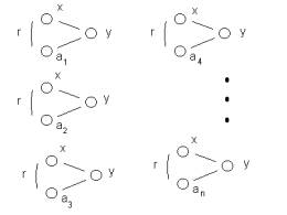
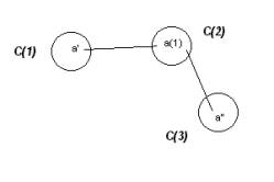
Figure 7: A chain relationship between a(1) and a(n)
The events in Figure 3 have a specific nature if the first and second columns are (1) attacker locations { x, a(1), a(2), a(3), a(4), . . . , a(n) } and (2) defender location, { y }.
We have seen two different interpretations of a chain relationship of this type given these two columns in the data mart. The first interpretation is about the identification of a Trojan and the consequent use of this knowledge by the attacker. The second interpretation is about session hijacking.
So what is the different between these two types of events?
The first interpretation was the motivation for the example SLIP Framework that the demonstration (version 1.4) displays and navigates. A port scan, from an source a(i), is used to trigger a response from a Trojan existing at location y. Given a successful response from the scan, it is assumed that a(i) communicates off line to x and that x then addresses the same port at location y and establishes a session that in some way uses the Trojan.
A different source IP , a(j), is used against a different target IP – again denoted in Figure 3 as y. The identity of y is not used in the SLIP scatter gather and thus the fact that the y may change location is not accounted for. We create a category Y, of y locations and treat any member of the category without distinction.
y(i), y(j) is an element of Y à y(i) – y(j)
If in each case, a single IP is used once a Trojan is identified, then we have established the chain relationship. The source IP locations { x, a(1), a(2), a(3), a(4), . . . , a(n) } will form all or part of a prime core.
The second interpretation is quite a bit different, and yet has almost the same characteristics when put into the SLIP Framework. One form of session hijacking occurs when an SYN is sent from x to y but x is spoofing its location, using the location a(i).
Some considerable work needs to be done in order to catch a reply from one of the spoofed locations.
Rout traces will sometimes work, if the administrator has not turned off rout tracing. Then given the ability of catch the reply, the source must manage to guess the session id number. Here is where a vulnerability of the attacker occurs. The ability to guess the session id is completely dependent on there being very little time elapsed between the SYN and the ACK reply. A SLIP signature for this type of element could be the membership in E4 of the first example SLIP Framework.
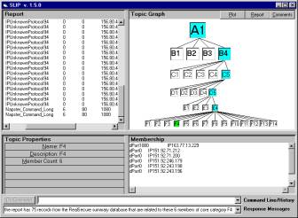
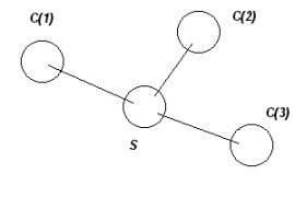
Figure 8: Five spoofed addresses chained to a port 1080 attack
Motivation: The motivation for creating a batch of test sets and examining the cluster cores, is to classify types of attacks from the patterns given in chain relationships within the pair table. These chain relationships are due to shallow link analysis. The clustering merely shows us where to look. The halting condition for clustering has been shown to be equivalent with a formal property about chain relations. So one has a computational foothold on the chains themselves. The chaining in turn reveals real, but non-specific linkage between data elements that exist in the data due to specific causes.