Event
Detection and categorical Abstraction
April 9, 2002
Copyright: Paul S.
Prueitt PhD, OntologyStream
Event
Detection and categorical Abstraction
April 9, 2002
Copyright: Paul S.
Prueitt PhD, OntologyStream
Introduction
The
objectives of this paper are to:
1. Demonstrate Shallow Link analysis, Iterated scatter-gather and Parcelation (SLIP).
2. Address the question of scalability.
3. Address the question of the development of a multi-resolutional Knowledge Base of categorical Abstraction (cA) in the form of event atoms, link-types and event compounds.
4. Indicate the potential use for SLIP and cA as a Synthetic Perceptional System for revealing Internet events and events that are composed from invariance in data.
In meeting these objectives, we shown that it is possible to develop a repository of abstract information through the use of categorical Abstraction (cA), and a theory of stratified complexity.
Stratified complexity is a theory of physical science, and has an exposition in the manuscript “Foundation of Knowledge Management in the 21st Century”. In this manuscript, stratified theory is developed using specific citation into experimental literatures from biology, cognitive neuroscience, and quantum mechanics.
One can use stratified theory to measure and organize the types of events occurring in the Internet.
Our software shows that these events are reducible to patterns and categories of patterns, and viewable as categorical abstraction. The categorical abstraction is produced in layers that correspond to use of computers (a) at the processor level, (b) as structural invariance recognized by software, (c) at the transport level between computer, and (d) at the level of use patterns (such as business logic.)
We have made an application of stratified theory to event detection via the categorical representation from structural invariance in data sources. We have shown that it is possible to reveal classes of invariance in arbitrary data sources, including computer code, text databases, and scientific data.
Data Set 1: In this example, categorical Abstraction (cA) is used to look at Linux behavioral data. Our data is a collection of 120,246 audit records from code sensors embedded in a Linux operating system.
Data Set 2: A small private Computer Emergency Response Team (CERT)-type commercial firm provided a data set with 65,535 records.
Data Set 3: A parsing program was developed to study the functional load of verbs and nouns within text units.
Section 1: Setting up
Our first data set is a collection of 120,246 audit log records from code sensors embedded in a Linux operating system. We start with:
·
Massive amount of data and
·
No identification of boundaries of events, event types, or occurrence
sequences.

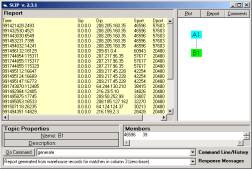
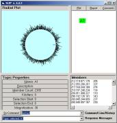
Figure 1: The SLIP Warehouse Browser
The first thing that we do is to apply a shallow
link analysis between two columns from the audit log.
1.
Shallow link analysis can be deepened to include any well-formed formula
over a first order predicate logic where the logical atoms are computer
addressable.
2.
Shallow link analysis is sufficient for a clear perception about event
types occurring in the Internet.
The
formation of our logic system is related to a foundational difference between
logics based on logical positivism and the logics based on stratified
theory. The logic system must support
variations in conjecture that are made are the axiom level.
The
two central aspects of this work are
(a)
The transfer of tacit
knowledge from analysts into the structure of agile and stratified conjectural
logic, and
(b)
The extraction of redundancy
during useful variations of agile stratified conjectural logic.
Our
work shows that almost the same view of the audit record is developed using
quite different conjectural logic and using variations of the instrumentation
and sensor configuration that is part of the cause of the audit log. The question of variation in conjectural
logic then is seen to be of importance as a means of studying how human might
use cA as a supplement, or replacement, to data mining, statistical pattern recognition
and self-organizing feature extraction.
The
same view is possible via two different conjectures because what is being
viewed, the data, is the same regardless of the conjecture used. Of course instrumentation and sensor
variation will change what is being viewed.
But that which is being viewed is part of the cause of the audit
log.
For example,
in Figure 1 we select source port
as the origin of atoms and destination
port as a non-specific/specific relationship.
The
specific relationship has meaning to the link-types. The non-specific relationship has meaning to compound types that
are formative ontology where the specific relationship has been set aside.
Interpretive
acts are required (by humans – not computers) to shift between the two levels
of structural organization. The
structure then, in and of itself, can be said to be “complex” in that the
structure has two meanings where the origin of meaning is completely different
and perhaps not coherent with each other.
In
Figure 2, 1,456 SLIP atoms are scattered to and then self-organized, via the
non-specific relationship, on the surface of a two dimensional circle. Atoms and link-types are abstractions
developed from high-speed data aggregation processes. The self-organization identifies compounds that are higher-level
structural patterns. The specific relationship
remains a local structural feature of the data, but we have now also a new
global organization of structure.
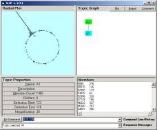
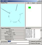
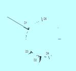
Figure 2: The SLIP Technology
Browser.
Once the SLIP atoms are scattered to the circle, one may command the browser to self organize into clusters. In less than 20 seconds around 100 million machine cycles are used to produce the emergent topology seen in the left windowpane of Figure 2. The command 123,128 -> B1 brings 1133 of these atoms from the spike cluster into a category B1.
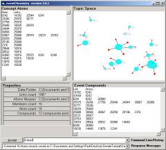
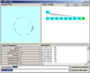
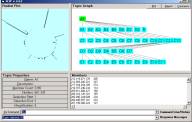
Figure 3: Category randomly scattered
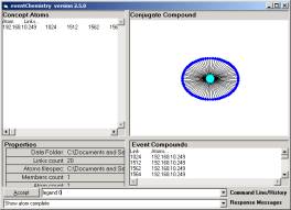
Figure 3 shows a small category randomly scattered and then rendered in the Topic Space window of the Event browser. The properties area shows that there are 12 simple compounds in the category. In the Event Compound window, pictured in Figure 4, we show the largest simple compound in this small category. Six of the atoms are involved.
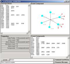
Figure 4: Category Compound
Annotation assists the task of shared human knowledge. Working notes can be annotated and made part of the event type history. For example, we find that the source port 30067 has three (un-identified) destination ports related by the conjecture. Source port 26980 has three un-identified destination ports. This simple compound has six valances and each is connected to one of 11 simple compounds. The meaning of this cA is held in the mind of a human.
In looking for ways of representing tacit knowledge, one can look to the formation of a synthetic language that is conditioned and co-evolved by the computer and by human communities of practice. By synthetic language we mean a language that is co-developed by computer processes and is about the type of invariance that occur completely inside of a computer process.
In the evolution of a synthetic language, human tacit knowledge is involved in three ways:
· The instrumentation and sensors are configured in a certain way. Humans must determine how this is to be done.
· A rich set of conjectures has to be figured out so that event atoms and link-types are produced as categories
· The formative process of producing an event compound may be influenced by feedback and user or expectation profiles
Ultimately what we are after is an emergent and living human/computer language system that is about abstractions and specific reification of these abstractions in specific data, and provided meaning by a human community.
The language system is one level of organization of meaning. But this single level of abstraction and meaning has a substructural support from a quite different level of organization of meaning (the specific relationship used originally to define sets of atoms and link-types). The tokens of this synthetic language are the set of object compounds that are defined from these three uses of tacit human knowledge.
The human community provides the meanings of the object compounds and the memory of language meaning is maintained by human minds, in exactly the same way as natural language is maintained by human minds.
The set of cA objects can be used as a query language into the original data, or into data that has a quite different origin. In Figure 5 we show the report generated from the original data for the category in Figure 4. Why can the compound map retrieve data from other data sets different than the original data? The answer is that the compound map is a visual rendering of categorical Abstraction existing at two levels of organization of meaning. The cA is drawn from a data set, but once obtained can be modified and made to retrieve from another data set.
By analogy, one can use the word for “tree” to refer to a specific tree, and then later use this same word to refer to a quite different tree.
Report generation uses a small-specialized In-Memory Holonomy Object (I-MHO). The query language for the compound maps is integrated with these I-MHOs. So the “theory” that we have is fully realized in existing and simple algorithms.
The algorithms are simple, are held to be proprietary, and are held to be extensible into as yet undiscovered theory and algorithms. It is like pure mathematics, in this regard.
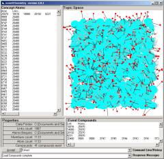
Figure 6: The
1123 atoms of category
By double clicking on the B1 node we scatter the 1133 atoms into a three dimensional space (Figure 6).
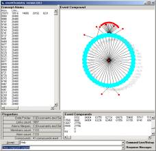
Figure 7: The largest of 41 categories
We know from a theorem, on prime decomposition of SLIP compounds, that 12 simple compounds can be assembled in such a way as all of the compounds are linked and there are no links that are left open.
Figure 7 is one of only three very large simple compounds representing the behavior of a Linux operating system. This compound is one of the self-organized features of the atoms in Figure 6.
Using a small downloadable software package, the reader is
able to see the categories in B1 and use the up and down keys to quickly view
them. So we should now do a
tutorial with this
software.
The tutorial begins with a Data folder that consists only of a 1,069 K log file and the OSI Browsers. These files are zipped into a 480K file called pre-cdkb.zip.
Unzip pre-cdkb.zip into any empty folder. You will see the folder shown in Figure 10.
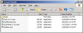
Figure 10: Pre-CDKB Tutorial
The Splitter has already been used to reduce the size of the Linux data set to 1/6. The following steps can be repeated so that you also discover what is available from this 1/6 of the original data set.
The
fact that Internet events are often fractal expressions of a small set of tools
implies that a relatively small number of sensors, and slow sampling rates, can
be deployed to measure the formation of cA over time. Of course, selective attention to events will produce faster
sampling and the engagement of exploratory instrumentation. The work on
selective attention ties the Synthetic Perceptional Systems concept more closely to cognitive neuroscience. This citation to existing scholarship is
detailed in the book: “Foundation
of Knowledge Management in the 21st Century”.
Lets
look at formative rates of cA, more closely.
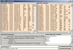
Figure 9: The Splitter
Using the Splitter, one selects the modulus n to produce a random sample of size 1/n. The Splitter takes every nth line and writes this line out to a new file. The residue m moves the beginning of this process to the mth line. We develop a 3/6 split starting with the third line and taking every 6th line into a new file.
This file must be renamed to datawh.txt to start the new study.
We have already done this in preparing the tutorial’s data file. You may close the Splitter browser. Double-click on the SLIPWhse.1.2.0.exe to open the Warehouse Browser.
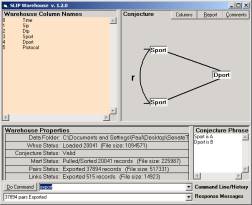
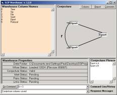
Figure 11: Creating pairs and exporting
You will see a list of the column names. Type in a = 3 and b = 4 to set the analytic conjecture as seen in Figure 11. Now command Pull and Export to produce the files needed by the next browser. In the command line of the Warehouse browser, we may type help to see the commands that are available for this browser.
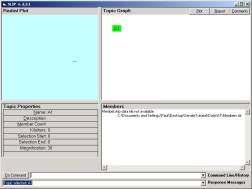
Figure 12: Import data and Extract atoms
Now double-click on the SLIP.2.3.1.exe to open the Core Technology Browser. All of the OSI browsers remember how the windows were positioned last time this browser was opened. One can move the different parts of these browsers.
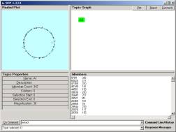
Figure 13: Click on node A1
However, on start-up your browser will look like Figure 12. Later versions of the Browser, renamed “SLIPCore”, require that the user issue a load command after the import and extract commands. Once these commands have been issued, one should then click once on the A1 node. The 342 atoms are scattered to the circle in Figure 13. This is compared to 1456 atoms for the full data set in Section 1. The ratio 342/1456 is about 1/4.
Now double click on the A1 node. The eventChemistry browser is launched and receives the object content of node A1. When compared to Figure 6, 30 compounds rather than 41. We reduced the size by 83% and yet the number of categories is reduced by only 27%.
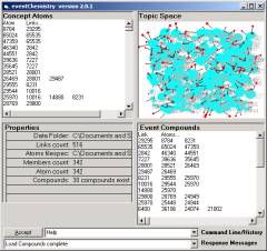
Figure 14: Node A1 in the event browser
In the Event Compound window scroll down (or use the down arrow) to find the 0 link (first column). Click on that line to produce the event map seen in Figure 15. Now compare this event map with Figure 7.
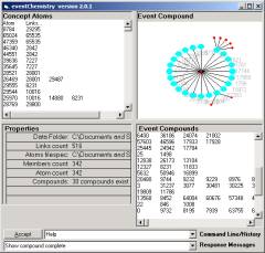
Figure 15: The eventChemistry Browser
Once a human sees the similarity, small variations in this pattern is immediately seen by the human mind as “the same”. This priming of awareness is the route into the formation of the synthetic human/computer language.
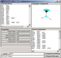
Figure 16: Conjugate Compound
One can navigate through the 30 event maps in this event knowledge base. Move the mouse over the map until you are over one of the red dots or one of the blue nodes. The cursor will change shape. Click.
The maps center either on the link or the atom. So when one starts we have a link, say link 0, which organizes the atoms that have that link as a valance.
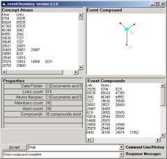
Figure 17: Navigating the complex graph
In this state the map is hot at the atoms. Move the cursor over any one of the atoms. The cursor will change shape. Click.
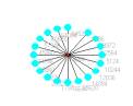
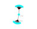
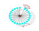
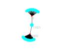

Figure 18: A transitional element between two
major events
If you find the 256 atom (having two valances) and click the eventChemistry will produce Figure 16. This map is centered on the atom rather than the link and shows that atom 256 has three valances { 0, 211, 35 }.
Clicking on either 211 or 35 will produce an atom with three links.
The structure of the two atoms is the same, but the details are different. Clicking on 0 will move the view back to what we see in Figure 17.
In Figure 18 we see two transitional elements between the three major events occurring in a Linux kernel.
Navigation and full visualization is still being thought through. We know from the theory that there are some interesting problems that have yet to be solved.
But not knowing completely how to use cA is not surprising, given the nature of the discovery. The browsers are like microscopes. They are used to find cA objects and linkage between cA objects. As discussed above, the specific linkage used, in an examination of the data, depends on the conjecture.
Once an appropriate conjecture has been established then specific clusters of atoms will indicate events. What the events are is a question of interpretation, but the presence of these events is not subject to question. There is structure in what is in the data, and this structure is what is rendered in the event window.
Our observation has been that cA is atypical to statistical analyses of invariance. Both can be used together to support analysis. It is also new, in the sense that the uses of cA have been developed only just a little.
Please call Dr. Prueitt at 703-981-2676 if your have any questions about the tutorial.
Section 2: The Internet Trunk data (Data Set 2)
The SLIP and eventChemistry Browsers are investigative tools directed at identifying events that are distributed in location and time. Once these events are identified then the **signature** of the event can be coded in a distributed Intrusion Detection System (dIDS).
We have shown evidence that the OSI propriety stochastic processes are fractal in nature. This evidence points to a deep result that is being developed as part of the logio-mathematical foundations to cA.
There are some fine points about the fractal nature of large data sets. Like a hologram, the resolution is affected by taking only small pieces of the hologram. In the small pieces one can still see the same limiting distributed. Like an image compression fractal, low resolution on the limiting distributed can be computed to provide an conjecture about what the higher resolution would look like if the data where available.
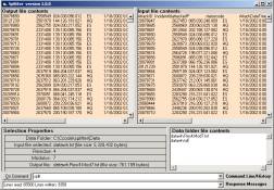
Figure 19: The Splitter Utility
The notion of splitting the data is simple. One can specify a fraction between 0 and 1 such as 4/7. This will produce a data set 1/7th the size of the original by starting at the (4+1)= 5th record and writing every 7th record to a new file. This new file is a splitting of size 1/7.
One can see this in Figure 19.The focus can be used to extract relevant data from new data sets. This extraction process is a simple data mining process.
In Figure 20 we have the limiting distribution of a 1/4 split of a 5,205K data set. The first layer (B) has 8 clusters, only 2 of which are formally prime. Further decomposition ends up producing 9 primes in level C, 6 primes in level D and 11 primes in level E. Theory indicates that the total number of primes is an invariant of the splitting process. We see a total of 28 primes of size greater then 1.

Figure 20: 28 primes of the 1/4 split of the original data
The splitter was used to create a 1/9 split on the 5,205K data set. The new datawh.txt has size 592K and has is 7241 records.
This file was placed into the folder “Data” with the three SLIP Browsers:
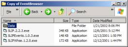
Figure 21: A folder containing the SLIP Browsers and the Data folder
The folder shown in Figure 21 is the standard set up for using the SLIP Browsers. The only file in the Data folder is the “datawh.txt”. As the browsers are used, additional files will be created within the Data folder.
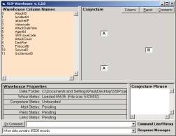
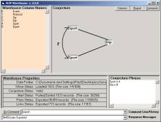
Figure 22: Initial state of the Warehouse
The first thing to be done is to open the SLIP Warehouse Browser (Figure 22).
The analytic conjecture specifies the atoms as attackerIP addresses. The original data set is raw data from around 100,000 firewalls so a large number of different attackerIP are reasonable. Previous studies indicated that the Destination Port is an excellent way to categorize types of events (whether attacks or other types of events).
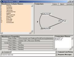
Figure 23: The development of an analytic conjecture
Flipping the analytic conjecture so that Destination Ports are the atoms and attackerIPs are the links will reveal additional information about the events of interest in this data set.
a
b
Figure 24: The initial (a) and limiting (b) distribution of the 2385 attackerIPs
a
b
Figure 25:
The parcelation of the first level of the SLIP Framework
But let us look first at the distribution of attackerIPs as organized by Port information.
Again, our stochastic theory predicts that if we do any other splitting that the limiting distribution will be very similar to the distribution seen in Figure 24 b.
Using the “bracket function”
a, b -> B1
we parcelated the limiting distribution into 8 categories and the residue. These are labeled in Figure 26 a.
a
b
Figure 26:
In Figure 26a we have the limiting distribution of the C12 node. C12 is derived from the cluster B7, which from inspection of Figure 24b, one can see a diffuse category with specific substructure. By randomizing and computing a limiting distribution we reveal this substructure as clusters.
Section 3: On the question of a knowledge base
In
this section we address the question of the development of a knowledge base of
categorical Abstraction (cA) composed of link-types, atoms and event compounds.
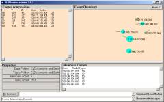
Figure 27: The random scatter of the 6 atoms of category E5
An eventChemistry (eC) is defined to be a set of rules that when applied to a simulation of atom dynamics produces a resolution where all of the common valances are fulfilled. To fully explore the eC we have developed a simulation environment.
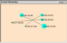
Figure 28: An event compound showing the common use of port 123 by exactly six IP addresses
By using the simulation environment it is possible to build a special information base consisting of event compounds and event atoms and descriptions and annotations of these compounds and atoms. These information artifacts are shared within a community.
In Section 1 we discussed the requirement that tacit knowledge be expressed in conjunction with the evolution of a set of symbols. Three important types of knowledge sharing are possible.
· The instrumentation and sensors are configured in a certain way. Humans must determine how this is to be done.
· A rich set of conjectures has to be figured out so that event atoms and link-types are produced as categories
· The formative process of producing an event compound may be influenced by feedback and user or expectation profiles
For the cA to be utilized the language must develop that allows humans to interact with work task and with the symbol system.
For example, the compound in Figure 32 is not representing a specific event. It represents a category of events – those that are using port 123. One may write queries against the FTP log traces and ask for all records where the port was 123. The software supports this. The result is 872 records has port 123 as the source port.
The invariance in the 872 records is condensed to a simple picture. The human can look at the picture and make associations between this picture and other pictures that have been developed and placed into an information base consisting of event compounds and event atoms and descriptions and annotations of these compounds and atoms. This is just one step in the normally complex process of sharing knowledge with the help of a natural language within a community.
Knowledge sharing within a trusted community can compete with the pool of variations that might be introduced as a means to test the strength of the Internet security mechanisms. The current SLIP and eventChemistry tools are reactive and predictive. We see the activity of individual hackers and communities of hackers, we use the semiotic language with cA objects, and as a consequence we can take appropriate action. The Knowledge Base, about compounds and atoms, evolves with the introduction of new tools into the hacker community and with new exposures of vulnerability.
VisualAbstraction renders all of the data into categories, where each category is representing all of the elements that are exactly the same. The pictorial icon is that set of categories with all of those relationships, and only those relationships, that are in the original data.
We “see” the invariance in the data, and relationships between the invariance in the data and we see all of this invariance all at once. Again, the invariance seen is due to (a) there being structure that is in the data, (b) the instrumentation and sensor settings, (c) the conjecture that produces atom and link categories, and (d) the event chemistry used to form compounds or links and atoms.
Invariance can be defined as being exact, or being exact after the application of a specific transformation. For example, “here” and “ehre” is the same after a juxtaposition of the first two letters in one of the two words. One can replace the notion of exactly the same with the notion of similar in this specific way.
There are variations in the substance of mental abstractions. The positive integers, for example, have an exact correspondence with things that occur in the natural world. But do negative numbers have an exact correspondence with something that occurs in the natural world? We have things that are three in number. But do we ever we have something that is minus three in number?
Correspondence to the things in the natural world is fleeting. And so we find that the relationship between those mental abstractions, which are about numeration, does not lead always to an absolutely consistent framework.
One should expect that work on visualAbstractions have similar difficulties.

Figure 27: One of the m/9, where m < 9, limiting distributions
In Figure 27 we have a limiting distribution over a second splitting of the original dataset. The original data set has 65,535 records. Each of these two splitting have 7,281 records. The most critical point to recognize is that we change the starting position and then take every 9th record and place this record into a new file to form the two splitting. Thus the two data sets are physically “split”. No two data sets have a single record in the intersection.
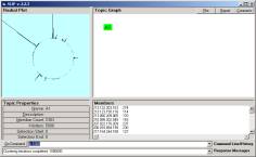
Figure 28: A second of the m/9, where m < 9, limiting distributions
There is a great deal of work that can be done here to formally exposit the evidence that the limiting distributions of splittings are a fractal type (holonomic) representation of the entire original data set. The first thing to notice is that the positioning of the clusters will vary as well the immediate surroundings of the clusters. We saw this in the early papers on SLIP distributions. However, the decomposition of these clusters will produce a unique SLIP Framework.
Early in the development of the first software, we approached the issue of Framework generation using a program that would cluster and then identify clusters of various types. Each cluster would be brought into a category and this category’s atom would be re-clustered to produce smaller clusters. A halting condition was defined and the notion of a unique decomposition of a set of atoms into primes was developed.
A prime is a category with a linkage relationship that will bring the elements of the prime to the same location during the stochastic process of scatter gather. The data used is a 1/9 splitting of the original data. The event compound for this small prime is Figure 3a. We then took a 1/50 splitting of the original data (Figure 29).
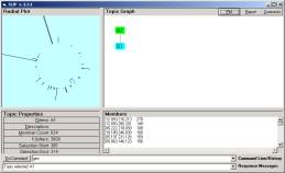
Figure 29: One of the m/50, where m < 50, limiting distributions
In Figure 29 we identified one of the atoms from Figure 28 to be part of a small category (marked by the blue bracket in Figure 4). On closer inspection we found the cluster had the five atoms.
The point of this is that an event found using 1/9 the data is almost completely found using only 1/50th of the data. We would also find this same event in any of the other 1/9 splittings.
In Figure 29, we see the large spike at about 100 degrees, and a second large spike at around 170 degrees. By looking in Figure 27 and Figure 28 one see similar structures. One of the differences between the 1/9 distributions and the 1/50th distribution is the degree to which small groups break away from each other. This is perhaps expected, as the background noise is reduced where as the primary patterns are seen because sufficient data still exists to produce the abstractions. We will loose many of the small events. However the larger events will be more clearly seen.
The formation of complex compounds has presented
considerable challenges. One
manifestation of this challenge is the simulation environment that we have
called the object space. The object
space is rendered in the upper level window of the event browser.
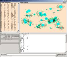
Figure 30: The first rendering of atom objects in the SLIP Object Space
The first rendering of atom objects in the SLIP
Object Space was made on December 17th, 2001. A “bag” of atoms is identified. Using the Event browser, these atoms are
randomly scattered into a 3-D space.
The Event browser remembers the positions of each of these atoms. Individual atoms can be moved. The size of an atom is used to represent its
z-axis as distance from the user.
Since December 2001 we struggled with a number of
visualization issues. We produced software and developed new theorems and
conjectures.
For example in Figure 31a the Dport (destination
port) organizes the Sport (source port).
The set of atoms is that set of Sport values that become paired in the
conjecture. A set of Dport values
becomes the abstractions that link these atoms together into compounds.
 a
a
b
Figure 31: Dual Analytic Conjectures
In Figure 31b we have the dual (sometimes called the
conjugant) conjunction.
Is the set of links from Figure 31a the same set as
the set of atoms in Figure 31b? Is the
set of atoms from Figure 31a the same set as the set of links in Figure 31b?
To answer these questions we developed an object
model where the atoms, links and compounds each are addressed separately.
Section 4: Linguistic Functional Load
Consider a set of concepts,
C = { ci }
where the index i is from the integer 1 to the integer n.
Consider that we have a procedure for guessing if ci is expressed in tk , where
{
tk } = T
is a set of text elements and k is a second index.
Select { di } = D , a subset of C , to be the “organizing set”. Now for each d* in D find all
ci in C such that m( ci , d* ) < q .
The metric function m is any distance or closeness function.
Define a set of pairs { ( ci , dj ) } where ever m( ci , d* ) < q . Create a tab-delimited line in an ASCII text file for each pair.
Import this text file into the SLIP Data-warehouse Browser. The Browser’s import process develops several In-Memory Holonomy (I-MH) objects. The I-MHs are required for fast stochastic processing.
The import is fast, and once completed the user can develop either one of the two possible analytic conjectures. (Note: If the import file has more than two columns then any two of the columns can be selected (in either one of two ways) to produce a different analytic conjecture. But the mapping of functional loads, on concepts in text collections, using the metric function m produces only two choices.)
Any first order predicate logic, defined over the set of columns types, can be used to produce an analytic conjecture. Once produced, the output data will be in the same form as in the simple case.
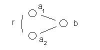
Figure 32: The non-specific relationship between the
atom a1 and a2
In the simplest form of an analytic
conjecture, two values from the first column, designated in the Figure as a1 and a2 , are paired if
the associated value, designated in the Figure as b, in the second column is the same.
Formally we have:
( a1 , b ) + ( a2 , b ) à < a1 , r, a2 >
where
r is the non-specific relationship.
This non-specific relationship is used in the stochastic process
provided by the SLIPCore browser.
At this point, we have information at two levels. The first level is the raw data linked by the non-specific relationships. The second level is a set of abstractions that represent invariance exposed by the non-specific relationship.
The analytic conjecture is about a non-specific relationship between pairs of data invariance. The non-specific relationship is NOT specified in the data itself. The non-specific relationship is used to produce an emergent metric over the data invariance.
The
pair-wise metric, when convolved via a stochastic process, is an open inference
about the activity and motivations that are the external causes (causes from
outside the computer systems). This
openness is available for manipulation by the expert by the way that data is
selected, by the way the analytic conjecture is specified, and in the way that
derivative compounds are produced.
It is noted that the non-specific relationship, r, becomes a global pair-wise metric. We integrate (in general terms this is a measure dependant stochastic convolution) over the entire collection to produce a limiting distribution to the stochastic process. The local pair-wise metric is transferred to a topology on the set of all abstractions (atoms, links and compounds).
One
can also see that the pairing
process in the analytic conjecture specified a specific relationship. The b value induces both the non-specific
and the specific relationship. In
stratified theory, the non-specific relationship and the specific relationship
are not the same. The non-specific
relationship is used to induce a global sense of what is close to what. The specific relationship is a local relationship.
( a1 , b ) + ( a2 , b ) à < a1 , b, a2 >
One way to specify a metric function is to check for co-occurrence, within the same sentence, of a noun with any verb, or a verb with any noun.
Define
m( ci , d* ) < q
if and only if the concept ci , d* both are judged to be present in the same sentence.
There are issues regarding automated similarity analysis and the definition of a passage in literature. The similarity analysis must be situated so that the quite natural variation of intent by a human is captured when possible. Moreover the notion of the boundary of a passage should not be merely the marking of a contiguous line of text. Passages are bounded by intent of writer and the interpretation of the reader.
The set of concepts can be defined to be the union of the set of nouns and that set of verbs found in a text collection. This is a guess, but one that has some utility.
This is what was done in our study of the concept functional load in text collections.
A third level of abstraction occurs when we look at the resolution of linkage into compounds. The simplest, but by no means the only, way to have such third level abstraction is to represent the functional load of the abstractions corresponding to the data invariance exposed by the conjecture.
Functional load
The set of pairs produced from a SLIP Analytic Conjecture defines a set of abstractions called atoms and a set of abstractions called links. The stochastic process produces a third set of abstractions called compounds.
Let
S = { <
aj , r, ai > }
be the set of all pairs of the first column elements that have a non-specific relationship, r, between the pair.
Let
A = { ai | ai appears as either the first or the third part of the elements of the set S }
and let
L = { b | b appears as second part of the elements of the set S }
A is the set of atoms and L is the set of links. These are abstractions, similar in nature to other useful abstractions such as the counting numbers or the periodic table from physical chemistry.
The clustering of the set of atoms is not necessary in order to define the functional load. The clustering is called Parcelation in the SLIP terminology, since the set A is parceled into separated categories. During this process, a useful notion of a prime category is developed and some theorems developed and demonstrated. Parcelation and functional load are related by this formal construct.
We define the functional load for either an atom or a link.
Let
Ab = { ai | ai appears as either the first or the third part of those elements of the set S that have b as the specific relationship }.
Ab
is defined as the functional
load of the link b.
Let
La = { b | b appears as the second part of those elements of the set S that have a as the either the first or the third part of that element }.
La
is defined as the
functional load of the atom a.
The process of mapping the functional load of concepts, as expressed in text, is a specific application of a more general data mining and information development. This process relies on co-occurrence of patterns. It is assumed that the original of the data and the meaning of the data are what is the target of investigation.
For example, we have been interested in mapping the communities of hackers and inferring the motivation.
The most general setting requires that
1. Data be acquired that samples consequences of hacker activity
2. Link analysis has sufficient strength to bring a window of observation to bear on the activity.
3. Some predictive modeling is made available to individuals who are trying to understand the hacker activity
4. Some form of community wide knowledge management system is made available.
 a
a
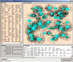
b
Figure 33: The version 2.3.1
Technology Browser and the version 2.0.0 Event Browser
Once atoms and links are defined, we produce
transformations of the atoms and links.
At first we approached this in a far more complex way then needed. We kept coming up against the halting
problem. By this we mean that a next
step, in the transformation, was any one of a number of choices and the outcome
depended on the order in which the choices are made.
We figured that a scatter-gather type process would
overcome the need to make decisions.
Such a process will make such a selection. During the month of December 2001, we could not get a complete
handle on the code issues.
We then represented the links and atom information
is two separate windows and allowed a single link to be selected. What we found was that in event chemistry
for data invariance, that the stochastic results and deterministic results are
in fact the same. Why? The answer is that, unlike the world of
non-computer-addressable subject; the computer-addressable subjects are always
completely reducible to a set of well-defined atoms.
We end this section with another short
tutorial. The download zip file has text data and is 585 K.
Unzip this file into any empty folder. This
will produce the following folder contents:
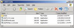
Figure 34: The unzipped contents of the demonstration
download
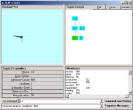
Double clicking on the SLIP.2.3.1.exe file will allow
one to double click on the C1 node to get the Event Browser to open and scatter
the 105 atoms from this category into the object space.
So how can we resolve these atoms into a single simple event
compound?
We know from theorems that category C1 is a prime. We know that a prime will resolve all of the
linkage (atomic valance) so that no link is left open. But how can we demand of the software that
such a resolution occur?
There are a number of good (and quite different
answers) to this question. For example,
we may first select any of the links and join all atoms having this link into a
simple
compound.
A simple compound is, by definition, only bound
together by a single valance type.
Remember that in linguistics, and in synthetic languages the linguistic
units have many ways in which a unit can be related to another unit.
Our first answer is pictured in the form of simple
graphs such as in Figure 35.
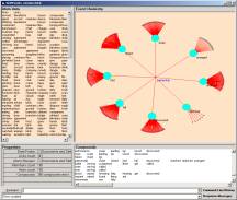
Figure 35: The functional load on
the concept “partnership”
In Figure 35 we find that the functional load of the
concept partner is the set of concepts:
{
share, seized, discovered, attacked, fold, fall, arranged, clutched }
The simple compound is rendered in the object space. The atoms are arranges in a circle and the
links that are not the selected link are shown going outward, as if not yet
resolved.
We know that ALL of the outward links are resolved
in the bag of atoms that is being considered.
But we do not show these atoms when reviewing the 105 simple
compounds. Typing “Extract Atoms”
will show all the atoms again.
An interesting simple compound is shown in Figure 36.
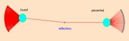
Figure 36: The simple compounds
“reflection”, with function load { found, presented }
So what to do?
How can we make a single compound that resolves all of the linkages in
all 105 atoms? And once this structure
is obtained, how can we view the structure and navigate into, and around, the
structure?
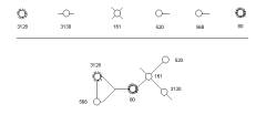
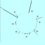
Figure 37: Early, hand draw, eventMaps for a small category
In Figure 37 we show an example of one of the early
hand-drawn eventMaps. Across the top we
have the individual atoms. In this case
there are only 6 so the display area is sufficient to display all of them. The compound is determined by which links
are actually shared. So atom 80 (the
e-mail port) and atom 161 share a common link.
Atom 80 shares a different link with both 3128 and 568.
Section
5: Event Detection
SLIP conjectures
can be any logical construction that involves a calculus on the names of the
columns, and on the contents of the column cells is a viable conjecture.
For
example:
The
value in the 5th column is x, y or z,
the
time is between p and q,
and
there is an occurrence of the value a, b, or c in the third column
after
the found value in the 5th column
will
produce syntagmatic units of the form < x, r, a >. Once one has a set of syntagmatic units, { < x,
r, a > }, one can define a set of
atoms and relationship types. One could
even define several types of atoms during the conjecture. The
x values and the a
values can be treated differently, for example, so that the r relationship have a temporal or
cause aspect.
Intrusion
Detection System (IDS) rules can be converted directly into a logical
construction that visualizes atoms and link-types. These atoms and links form a substructure for the production of
visual clues regarding the nature and variation of the IDS events. The IDS log file need not be the starting
point for visual abstraction.
Observationally,
we see that the conjectures produce object invariance that is driven by data
content. For each conjecture there are
between 3 – 10 major compounds and between 10 – 50 smaller ones. A conjecture can be applied, in real time,
to a data stream by building a dual-buffer where data is accumulated into one
buffer and the other buffer is used to build the cA. The dual-buffering architecture is commonly used in real time
compression and encryption streaming.
The
conjecture acts as a convolution over the data steam to produce a real time
imaging of exactly those events that are occurring in the data stream.
For example, we received 1833 snort records, and placed six
columns of this data into a datawh.txt file.
Figure
38: (source port, destination IP) conjecture
We
developed a (source port, destination IP) conjuncture.
"Source port behavior" is part of what is “in the
data” and can be useful as a means to point precisely at an incident. The source port will often be incremented
each time a packet is sent from the source IP address to the destination IP
address. So this should look like a
type of reverse port scan.
Port scans should be viewable using any one of several conjectures
such as (destination port, source IP), (destination
port, destination IP) or
the conjugant conjectures (source IP, destination
port), (destination port, destination IP).
"Source port behavior” can be used to illustrate the
operational properties of visual Abstraction.
In the conjecture (source port,
destination IP), the
destination IP organizes source port log file events. Compounds suggest how
source ports use the various destination IP addresses and how events are
reported to the snort log. The reader
is encouraged to look in the data set and investigate some of these compounds.
The issue of mental imaging and conceptual priming of the individual
experience of knowledge is a question of science.
The White
Hats (the good computer hackers) have many mental images of Cyberspace events,
and these mental images can be triggered by a visualAbstraction (perceptual
priming).
The
visual Abstractions can also be used to transfer domain specific tacit
knowledge from a White Hat (or CERT domain specialist) to someone else.
The human awareness, that is primed, will sometimes leads to the mental recognition that something is understood, or that something is "there" but not understood
For
example, our snort data set was given to the research group with the following
information:
" There were
some vulnerability scans and other things going on. "
To
investigate the vulnerability scans one should copy the snort2 folder (from
snort2.zip) and delete all files in the data folder except the datawh.txt
file. Then build a conjecture and look
at the compounds.
Figure
39: A possible
source port behavior event type occurring to Dip = 192.168.10.249
We will
take a slightly different approach. We
first filter the data to produce a datawh.txt file having only one specific IP
that appears to have been scanned.
Figure
40: Report
generated for all records having Dip = 192.168.10.249
Having
identified this potential port scan, we used the SLIPCore to manually bring the
single IP address into a category so that report
generation could
produce a file having only Dip = 192.168.10.249. Clearly some automation would be helpful here, but the data
structure is readily available for this type of query and retrieval.
Having retrieved the 193 records from the original dataset,
we now develop events using the (source port, destination IP) conjecture (see
Figure 41).
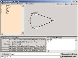
Figure 41: The conjecture (source IP, dest port) in
the query set
By inspection of Figure 42 we verify that there is only one
event compound, and that this compound is defined by the relationship to a
single destination IP, 192.168.10.249.
This single IP address has been passed information from 95
source ports. It is natural to ask if
the compete set of source ports are related to the same source IP, or are
related to source IPs that are known to have a common locus of control.
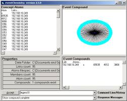
Figure 42: The view of the single compound having
the proper number (95) of atoms
One may
descriptively enumerate all event-types and to thus define what one means by an
event, taken in the abstract; and what is meant by each event, considered by
itself.
For example, when a port scan event appears to be starting we
will see an anticipatory object appear in the knowledge base interface.
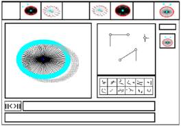
Figure 43: Mock up of a Knowledge Base
As the scan occurs, we should see the development of the scan profile. Other real time objects will be viewable, as will be incident histories. Variations from the typical object representation will be seen.
After the scan has been completed we may render the event at a higher level of organizational detail. Other technologies can be integrated with cA-based technology. Petri type models anticipate what might happen because of a scan of a certain type. Incident histories detail the behavior of a program of a particular type. Incident histories detail that a particular type of event has in fact occurred at a specific time. Thus technologies can be integrated into one system.
A four-layer taxonomy { bit stream, intrusion, incident, and policy } is seen in Figure 44.
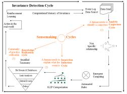
Figure 44: The first of four PowerPoint slides on SenseMaking
The facilitation of terminology development and use in a community of practice is an essential aspect related to the notion of a CERT center.
Once event types are identified then the knowledge base can be instructed to alert the viewer that specific events are present in the data stream. We may describe the "event" by name and short description and modify the object formation process to look just for this "object".