Index .
Tutorial on
eventChemistry and
Visual Abstraction
Knowledge Bases
February 14, 2002
Software
available at
http://www.ontologystream.com/cA/tutorials/download/pre-CDKB.zip
In
this example, event-Chemistry is used to look at Linux behavioral data. Our data is a collection of 120,246 audit
records from code sensors embedded in a Linux operating system. We start with:
·
Massive amount of data and
·
No identification of boundaries of events, event types, or
the occurrence sequence.
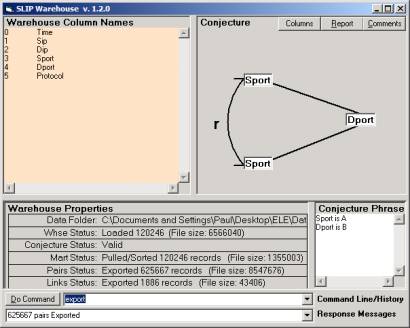
Figure
1: The SLIP Warehouse Browser
The first thing that we do is to
apply link analysis between two columns.
1) Shallow
link analysis can be deepened to include any well-formed formula over a first
order predicate logic where the logical atoms are computer addressable.
2) Shallow
link analysis is sufficient for a clear perception about event types occurring
in the Internet.
“SLIP” stands for Shallow Link analysis, Iterated scatter-gather and Parcelation.
In Figure 1 we select source port as the source of atoms and destination port as a non-specific/specific relationship.
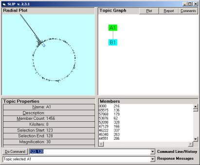
Figure
2: The SLIP Technology Browser.
In Figure 2 1456 SLIP atoms are scattered to and then organized on the surface of a two dimensional circle. Atoms are abstractions developed from high-speed data aggregation processes.
Once the SLIP atoms are scattered to the circle, one
commands the Browser to self organize into clusters. In less than 20 seconds around 100 million machine cycles are
used to produce the emergent topology seen in the left windowpane of Figure
2. The command 123,128 -> B1
brings 1133 of these atoms from the spike cluster into a category B1.
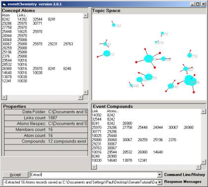
Figure 3: Category randomly scattered
Figure 3 shows a small category randomly scattered
and then rendered in the Topic Space window.
The properties area shows that there are 12 simple
compounds in the category. In Figure 4,
we have shown the largest simple compound. Six of the atoms are involved.
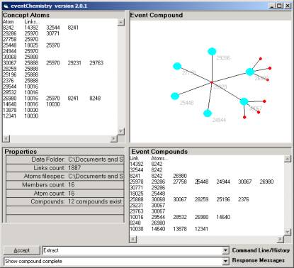
Figure 4: Category Compound
Working notes can be annotated and made part of the
event type history. We find that the source port 30067 has three
(un-identified) destination ports related by the conjecture. Source port 26980 has three un-identified
destination ports. This simple compound has six valances and each is connected
to one of 11 simple compounds.
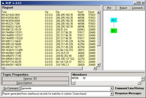
Figure 5: Report
generation
We know from a published eventChemistry theorem, on
prime decomposition, that all 12 simple compounds can be assembled in such a
way as all of the compounds are linked and there are no links that are left
open.
In Figure 5 we show the report generated from the
original data for the category in Figure 4.
The compound map can retrieve data from other data sets different than
the original data. Thus the
abstractions can be used as a query language.
The object space for eventChemistry is being developed strictly based on
I-RIB theory.
Report generation uses a small-specialized In-Memory
Referential Information Base (I-RIB).
The query language for the compound maps is integrated with a query
language for these I-RIBs.
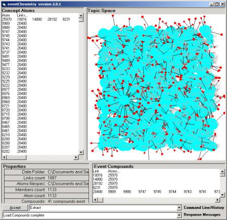
Figure 6: The 1123 atoms of category
By double clicking on the B1 node we scatter the
1133 atoms into a three dimensional space (Figure 6).
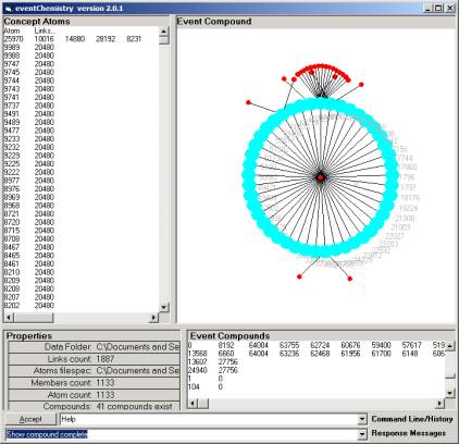
Figure 7: The largest of 41 categories
We know a lot about this category of atoms from
theory, for example, category B1 has 41 simple compounds. Figure 7 is one of only three very large
simple compounds representing the behavior of a Linux operating system.
Section 2: The tutorial
Using the small downloadable software package, the reader will be able to see a low-resolution version of the categories in B1 and use the up and down keys to quickly view them.
The study begins with a Data folder that consists
only of a 1,069 K log file and the OSI Browsers. These files are zipped into a 480K file called pre-cdkb.zip.
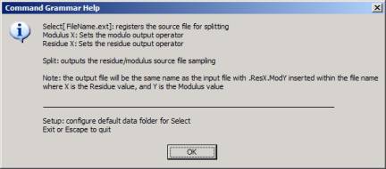
Figure 8: Help window
The fact that Internet events are often fractal expressions of a small set of tools implies that a relatively small number of sensors can be deployed to measure the behavior of the entire system. Lets look at this issue, more closely.
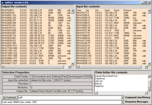
Figure 9: The Splitter
One selects the modulus n to produce a random sample
of size 1/n. The Splitter takes every
nth line and writes this line out to a new file. The residue m moves the beginning of this process to the mth
line. We develop a 3/6 split starting
with the third line and taking every 6th line into a new file.
This file must be renamed to datawh.txt to start the
new study. We have already done this in
preparing the tutorial’s data file.
Anyone can download the zip file from OSI or copy
this small file from one of the floppy disks, provided with our briefing
materials. Unzip pre-cdkb.zip into any empty folder. You will see the folder shown in Figure 10.
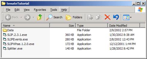
Figure 10: Pre-CDKB Tutorial
The Splitter has already been used to reduce the
size of the data set used in Section 1 to 1/6. The following steps can be repeated so that you also discover
what is available from this 1/6 of the original data set.
Double-click on the SLIPWhse.1.2.0.exe to open the
Warehouse Browser.

Figure 11: Creating pairs and exporting
You will see a list of the column names. Type in a = 3 and b = 4 to set
the analytic conjecture as seen in Figure 11.
Now command Pull and Export to produce the files needed by
the SLIP Technology Browser.
In the command line of the Warehouse Browser, we may
type help to see the commands that are available for this Browser.
Double-click on the SLIP.2.3.1.exe to open the
Technology Browser. All of the OSI
browsers remember how the windows were positioned last time this browser was
opened. One can move the different parts
of these browsers. However, on start-up
your Technology Browser will look like Figure 12.
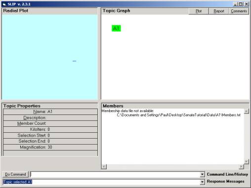
Figure 12: Import data and Extract atoms
In the command line one can issue the commands import
and extract. Import the data
from the folder and extract the abstractions called SLIP atoms. After a few seconds, the response message
will say Topic Map A1 is loaded.
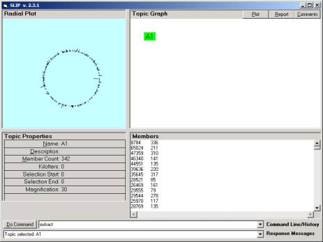
Figure 13: Click on node A1
You should then click once on the A1 node. The 342 atoms are scattered to the circle
in Figure 13.
This is compared to 1456 atoms for the full data set
in Section 1. The ratio 342/1456 is
about 1/4.
Now double click on the A1 node. The eventChemistry Browser is launched and
receives the object content of node A1.
We see that there are 30 compounds rather than 41. We reduced the size by 83% and yet the
number of categories is reduced by only 27%.
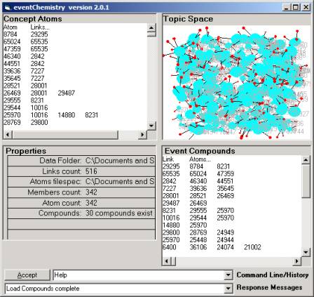
Figure 18: Node A1 in the event
browser
There are other measures of fractal and holographic characterizations
of abstraction and stochastic process involved in producing the atom and
compound abstractions.
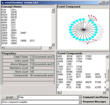
Figure 19: The eventChemistry Browser
In the Event Compound window scroll down (or use the
down arrow) to find the 0 link (first column).
Click on that line to produce the event map seen in
Figure 19. Now compare this event map
with Figure 7.
One can navigate through the 30 event maps. Move the mouse over the map until you are
over one of the red dots or one of the blue nodes. The cursor will change shape.
Click.
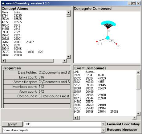
Figure 20:
The maps center either on the link or the atom. So when one starts we have a link, say link
0, which organizes the atoms that have that link as a valance.
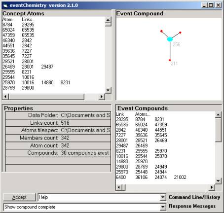
Figure 21: Navigating the complex
graph
In this state the map is hot at the atoms. Move the cursor over any one of the
atoms. The cursor will change
shape. Click.
If you find the 256 atom (having two valances) and
click the eventChemistry will produce Figure 20. This map is centered on the atom rather than the link and shows
that atom 256 has three valances { 0, 211, 35 }.
Clicking on either 211 or 35 will produce an atom
with three links. The structure of the
two atoms is the same, but the details are different. Clicking on 0 will move the view back to what we see in Figure
21.
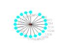
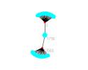
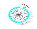

Figure 22: A transitional element
between two major events
In Figure 22 we see two transitional elements
between the three major events occurring in a Linux kernel.
Navigation and full visualization is still being
thought through. We know from the
theory that there are some interesting problems that have yet to be solved.
Please call Dr. Prueitt
at 703-981-2676 if your have any questions about this tutorial.